
Help Table of Contents
MetaWin
What is MetaWin?

3 is free, open source software for conducting the quantitative meta-analysis portion of research synthesis. It has been rewritten from scratch relative to earlier versions (see history). The new version is written entirely in Python, and the code is available on GitHub at https://github.com/msrosenberg/MetaWin. Single file executable versions of the software for Windows and Mac operating systems can be downloaded from https://www.metawinsoft.com.
A Brief History
(Rosenberg et al. 1997) was first published as a small, commercial piece of software that made meta-analytical calculations more accessible to the burgeoning research synthesis community, particularly in the ecological sciences, and helped introduce the use of resampling methods into the meta-analytic statistical repertoire (Adams et al. 1997).
Version 2 of the software (Rosenberg et al. 2000) was substantially expanded over the original version, easier to use, and more flexible and powerful.
The original versions of were written in Pascal and Delphi and depended on a number of commercially licensed packages. These developmental environments combined to functionally restrict the software to the Windows operating system and prevented any practial open source release as the software was otherwise uncompilable without these components. These also restricted further development and updates as the developmental components and systems gradually became incompatible with newer operating systems.
Despite these limitations, 2 continued to be regularly used and cited decades after its original release.
How to Conduct a Meta-Analysis
The purpose of this manual is to explain the software, not to teach the entire process of conducting a systematic review, of which the computational meta-analytic portion is only a part. Many books and tutorials have been written on the subject. One I would recommend (full disclosure: I was a contributor to the work) is the Handbook of Meta-Analysis in Ecology and Evolution, although there are many alternatives to consider.
The computational methodology in is largely independent of discipline, although different research disciplines do have their own eccentricities when it comes to analytical approaches, as well as particular challenges based on the sorts questions they tend to ask and data they tend to deal with.
Citation
The formal publication announcing MetaWin 3 should be used to cite the software:
Rosenberg, M.S. (2024) MetaWin 3: Open-source software for meta-analysis. Frontiers in Bioinformatics 4:1305969. DOI: 10.3389/fbinf.2024.1305969
Depending on the context, you might want to consider specifying the version (3.x.x) as part of your methods.
Suggestions and Bugs
Suggestions and bug reports can be submitted either through the GitHub site (https://github.com/msrosenberg/MetaWin/issues), which allows public and formal tracking of feedback.
For bug reports, please be specific about details including (1) what release of MetaWin were you using (listed at beginning of output or via ), (2) what Operating System were you using, and (3) as many specifics about the type of analysis you were conducting, including specific choices you made. We may secondarily request a copy of the dataset if we are cannot readily duplicate the bug.
General Interface
The primary graphical user interface (GUI) of is a tabbed window, with each tab containing a different type of information. A typical menu bar and toolbar are shown at the top of the window, while each tab has a unique toolbar on the left side. At the start, only two tabs will be visible, but a few others may appear as needed.
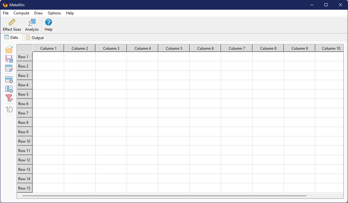
Primary interface in Windows. The layout in macOS is mildly different due to differences in the native OS.
Data Tab
The Data Tab contains a spreadsheet like view of data imported or created within . Data within the spreadsheet is not editable, that is, values cannot be changed or deleted. That level of manipulation must be done externally. The toolbar on the left side of the Data Tab can be hidden/displayed by choosing from the menu.
Importing Data
will only import text files, so data held in a traditional spreadsheet such as Microsoft Excel will first have to be exported. Any type of text delimiter can be used, although we recommend tab delimited as the simplest and most effective.
Data should be organized in a typical row × column table, with each row representing a study and each column a type of data associated with the study. Although not required, it is highly recommended that the first row of the imported file contain column headers. While less important, it is also generally recommended that the first column contain study labels.
Data can be imported into by choosing
from the menu or by pressing the
 button in the toolbar on
the left side of the tab. Upon doing so, the user will first choose the file to import using the system
file browser. This will be followed by the Import Text Options dialog window.
button in the toolbar on
the left side of the tab. Upon doing so, the user will first choose the file to import using the system
file browser. This will be followed by the Import Text Options dialog window.
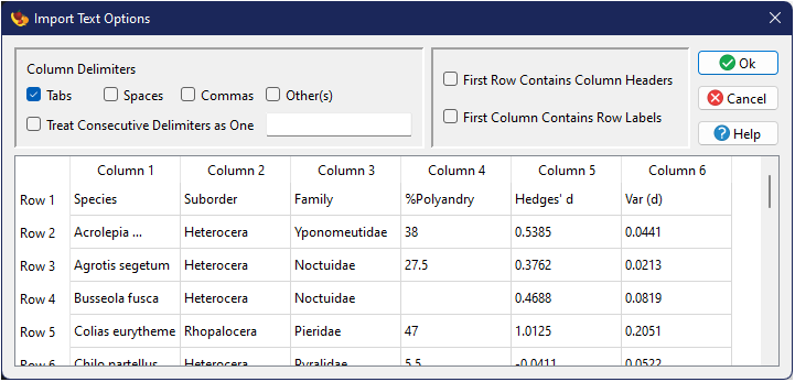
In this window, you can choose which delimiter(s) were used to separate columns within the file, as well as whether or not the first row and/or first column contains row and column headers, respectively. The remainder of the window illustrates a live view of how the data will be input based on the current choices.
Upon acceptance of your options, the data will be imported and displayed in the Data Tab grid.
Saving Data
If you have modified the imported data through the cacluation of effect sizes, this updated
data table can be saved to a text file by choosing
from the menu or by pressing the
 button in the toolbar on
the left side of the tab.
button in the toolbar on
the left side of the tab.
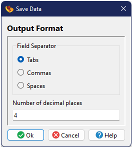
You will first be presented with a choice of column delimter, either Tabs, Spaces, or Commas, as well as the number of decimal places for real numbers, followed by a system file browser to choose the file name and location for the output.
Clearing Data
To erase all data currently loaded into memory, choose
from the menu or press the
 button in the toolbar on
the left side of the tab.
button in the toolbar on
the left side of the tab.
Filtering Data
Data filtering allows one to remove studies from subsequent analyses and graphs. The only operation which ignores filtering is the calculation of effect sizes (i.e., will attempt to calculate effect sizes for all rows, regardless of filtering choices). There are two ways in which studies can be filtered.
Filtering Rows
Individual studies can be directly filtered by right-clicking on the row header and choosing from the popup menu. The background of the row will change color (light pink by default) indicating the row is currently filtered from future analyses. Toggling the row again will remove the filter.
Filtering within Columns
Instead of filtering studies directly, one can specify values within a column to filter. To do this, right-click on the column and choose . This will open a new window with a series of checkboxes indicating all of the values found within the column. Uncheck those you want to exclude from the study. Studies with that particular value will be colored light pink (by default), just as with row filtering, but the column containing the value which is leading to the filtering will be given a different color (red by default).
Clearing Filters
Individual filters can be removed by repeating and reversing the process used to create the filter.
Alternatively, all filters can be removed by clicking the
 button in the toolbar on
the left side of the Data Tab.
button in the toolbar on
the left side of the Data Tab.
Data Options
Filtered Colors
Two colors are used to indicate rows of the data table that are actively filtered from subsequent analyses.
The first color generally indicates that the row has been filtered, while the second highlights specific columns
leading to the row filtering, when applicable. By default, these colors are light pink and red, but can be
customized by choosing and
from the
menu or
 and
and
 from the toolbar on the
left side of the Data Tab. If you change these colors, will attempt
to remember these choices the next time you run the program.
from the toolbar on the
left side of the Data Tab. If you change these colors, will attempt
to remember these choices the next time you run the program.
Decimal Places
By default, real numbers that appear in the data table will be displayed to 2 decimal places. You can change
this amount by choosing from the
menu or
 from the toolbar on the
left side of the Data Tab. Valid options are integers from 0–15. If you change the number
of decimal places displayed in the data table, will attempt to remember
this choice the next time you run the program.
from the toolbar on the
left side of the Data Tab. Valid options are integers from 0–15. If you change the number
of decimal places displayed in the data table, will attempt to remember
this choice the next time you run the program.
Output Tab
All textual output is displayed in the Output Tab, which will generally be automatically shown upon completion of an analysis.

Text displayed in this tab can be manually edited by the user and standard text edit commands, such as Copy, Cut, and Paste work through typical keyboard commands (e.g., Control-C, Control-X, and Control-V, respectively) or by right-clicking within the output area. The toolbar on the left side of the Output Tab can be hidden/displayed by choosing from the menu.
Saving Output
Output can be exported to a file by choosing from the
menu or
 from the toolbar on the
left side of the Output Tab. Output can be saved in three formats:
from the toolbar on the
left side of the Output Tab. Output can be saved in three formats:
- Plain Text: The plain text format strips all formatting (font size, bold, etc.) from the output and just saves the raw characters.
- HTML: The HTML format preserves all of the formatting as is; this output file is best displayed in a browser or converted by a word processor.
- Markdown: Attempts to preserve some of the output semantics through conversion to Markdown. Not all formatting will necessarily be maintained.
Note that all three formats are fundamentally text files, the difference is whether a form of text formatting is included within the files or not.
Output Options
Decimal Places
By default, real numbers that appear in the output will be displayed to 4 decimal places. You can change
this amount by choosing from the
menu or
from the toolbar on the
left side of the Output Tab. Valid options are integers from 0–15. Note that changing this value will
only affect future output; vales already written to the output will not be changed. If you change the number
of decimal places to use in the output, will attempt to remember this
choice the next time you run the program.
One exception to this choice are p-values generated from randomization tests. The number of decimal places used to display these values is automatically determined by the software based on the number of desired replicates.
Font
You can change the font and it's properties used in the Output Tab by choosing
from the
menu or
 from the toolbar on the
left side of the Output Tab. Changing the font will affect the entire output already displayed, not just new
output. Tables in the output are always displayed in a monospace font, regardless of the primary font chosen
for the rest of the output.
from the toolbar on the
left side of the Output Tab. Changing the font will affect the entire output already displayed, not just new
output. Tables in the output are always displayed in a monospace font, regardless of the primary font chosen
for the rest of the output.
Graph Tab
The Graph Tab will automatically appear the first time a figure is created by the software. Only a
single figure can be displayed at a time; each new figure will erase the previous one. To save a
figure, press the  button from the Graph Tab toolbar.
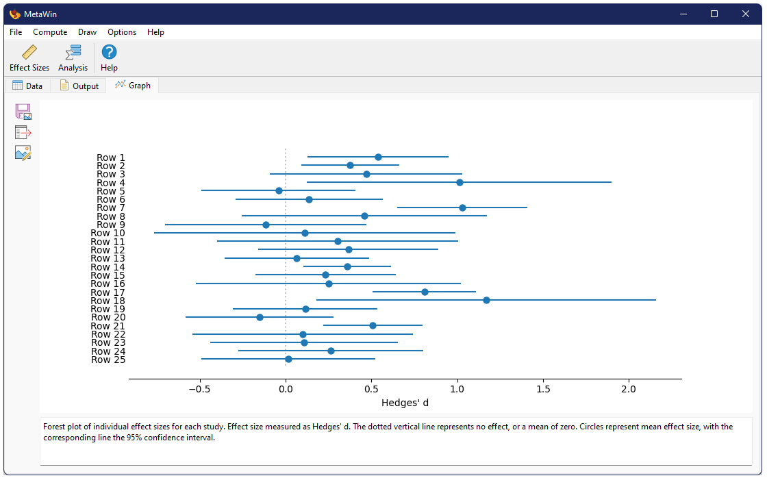
In addition to the toolbar and the figure itself, the Graph Tab has an automatically generated caption at the bottom of the window, based on the type of figure and the user decisions made in creating it. The caption will sometimes include citations to methods, when appropriate.
All of the underlying data making up a figure can be exported by clicking
 from the Graph Tab toolbar. This
could allow a user to redraw the figure in a program of their choice to give them greater control
over the precise figure style and form.
from the Graph Tab toolbar. This
could allow a user to redraw the figure in a program of their choice to give them greater control
over the precise figure style and form.
Editing Figures
Figures can be edited by clicking the
 from the Graph Tab toolbar.
This will bring up a window with a variety of options, depending on the exact elements that make
up the figure.
from the Graph Tab toolbar.
This will bring up a window with a variety of options, depending on the exact elements that make
up the figure.
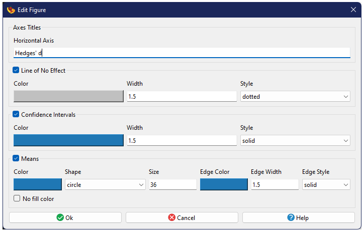
Most elements will have a checkbox next to their name (checked by default). Unchecking this box will hide the element when the figure is redrawn. Most of the editing options fall into just two major types of plot elements:
Lines
Many figures have lines of various sorts. Each type of line in a figure has three basic properties: color, width, and style. Styles include solid, dashed, dotted, and dash-dot.
Markers
Markers represent specific points drawn in a figure, such as those from a scatter plot. Markers have three basic properties and three extended properties. The three basic properties are color, size, and shape. Note that size is measured in terms of marker area. The color property for markers has an additional checkbox titled “No fill color”. Checking this box will eliminate the primary color the marker and only use the edge color, assuming the chosen marker is a filled marker (see below). Unfilled markers will turn invisible if the no fill option is checked.
Marker shapes fall into two basic categories: filled and unfilled markers. Unfilled markers are mostly, but not exclusively made up drawn lines (e.g., an X or a + symbol). Unfilled markers only use a single color. In contrast, filled markers (e.g., squares, circles, or diamonds) have both a primary color (the fill) as well as an outside edge. The edge not only has an independent color, but also has both a width and a style (identical to standard lines). These extended edge properties are ignored when unfilled markers are chosen.
The primary color property for markers has an additional checkbox titled “No fill color”. Checking this box will eliminate the primary color of the marker and only use the edge color, assuming the chosen marker is a filled marker. Unfilled markers will turn invisible if the no fill option is checked.
A Note on Captions
will autogenerate captions for each figure it creates, including references in some cases. As style elements of figures can be user edited, this creates a bit of a challenge for captioning, particularly as it relates to specifying color. Computers can generate over 16.7 million unique colors, most of which obviously do not have unique names. Although exact, specifying colors by RGB or hex number in captions would not be particularly useful. Therefore, whenever a caption includes a reference to a color, a color name is chosen by matching the specific color to the closest named color from a color name space. By default will use a set of approximately 1,000 named colors based on a survey done at xkcd. This set was chosen as the default primarily because of it's size. With that many crowdsourced color names, many may be a bit odd, so simply be warned if strange color labels appear.
Alternatively, one can choose to have color names in captions based on the X11/CSS4 color name space. This set is more formal, but only contains approximately 150 named colors and the names all lack internal spacing (so for example, "lightblue" rather than "light blue"). The following table compares the names of some of the more common default colors used in .
| Color | xkcd name | X11/CSS4 name |
|---|---|---|
| black | black | |
| silver | silver | |
| bluish | steelblue | |
| green | forestgreen | |
| tomato | crimson | |
| fire engine red | red | |
| pumpkin orange | darkorange |
Note that the names output by are based on finding the closest color that is named, such that the actual color used may not be the color precisely defined by the name space.
The option to switch between color name space is found under the menu.
Currently only line and markers description appear in captions. Line descriptions include only color and style (solid, dahsed, etc.), while markers include color and shape (two colors if the primary and border colors are different). Properties such as size and thickness are not included in captions.
Phylogeny Tab
The Phylogeny Tab is not shown by default because it represents a specialty analysis that may only be of interest to a subset of users. In order to activate the tab, one must first choose from the menu. This will open the tab, which allows a user to import a phylogeny as part of a meta-analysis.
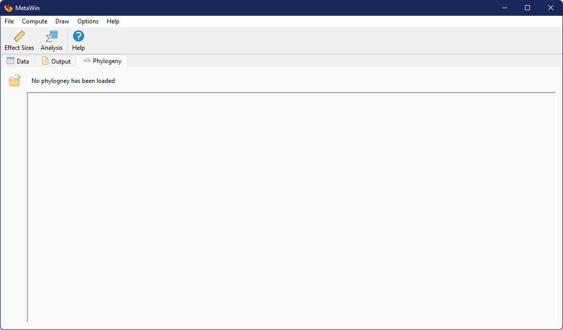
The Phylogeny Tab only has a single option, a Load Phylogeny button
on the left-hand
side of the tab. Pressing this will bring up the system file browser, allowing one to specify the
file containing the phylogeny to import. will only read text
files containing a phylogeny in Newick
format. The phylogeny is expected to be the first item within the file.
Upon a successful import, the top of the phylogeny tab will list the number of tips found in the imported phylogeny and a visualization of the phylogeny will be displayed in the remainder of the tab. This visualization is minimalistic and simply meant to allow a user to visually validate that the phylogeny was imported correctly. Currently, the entire phylogeny is squeezed into the window and thus may appear overly compressed if the window is not expanded.
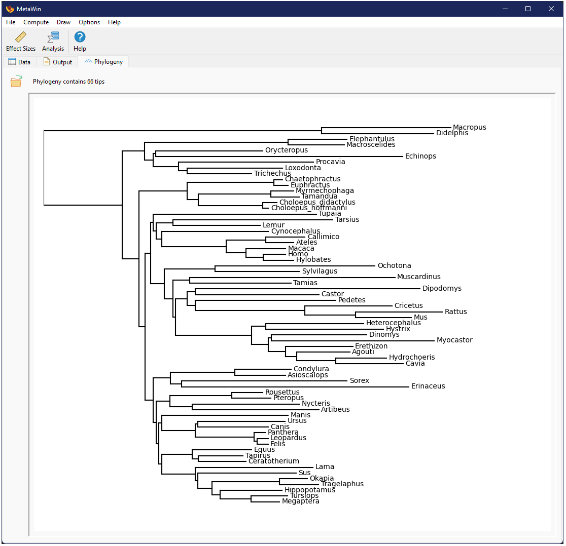
Once a phylogeny has been loaded into memory, the Phylogenetic GLM Meta-Analysis option becomes available.
Analysis Options
Significance Level
By default, significance levels for generating confidence intervals and certain types of tests are
based on a standard value of 5% (α = 0.05). This value can be changed by
choosing from the
menu or
 from the toolbar on the
left side of the Output Tab. Valid options are numbers between 0.01 and 1.0).
Note that changing this value will
only affect future output; vales already computed will not be changed. If you change the significance
level to use in the output, will attempt to remember this
choice the next time you run the program.
from the toolbar on the
left side of the Output Tab. Valid options are numbers between 0.01 and 1.0).
Note that changing this value will
only affect future output; vales already computed will not be changed. If you change the significance
level to use in the output, will attempt to remember this
choice the next time you run the program.
This choice also effects a few of the direct figures you can draw, such as Forest Plots and Normal Quantile Plots.
Confidence Interval Distribution
When determining confidence intervals around means using standard distributions (rather than a boostrap procedure), the traditional approach in meta-analysis has generally been to use a Normal distribution. In earlier versions of , we used Student's t distribution instead, because we thought it useful to account for the uncertainty in estimation due to the small number of studies often found in meta-analyses. With this new version, the user can specify which distribution they wish to use, with the Normal distribution set as default.
To change the distribution, choose the item under the menu, which will toggle between the two distributions. The current distribution is indicated by the icon to the left of the menu option (either a Z or a t), as well as by the text of the menu item which specifies the distributions being changed both "from" and "to". will attempt to remember this choice the next time you run the program.
The specified distribution is also listed as one of the user-specified parameters at the beginning of analysis output.
Additional Options
Check for Updates
By default, will automatically try to check to see if an updated version of the program is available when first opened. This option can be disabled under the menu. A manual check for an update can also be initiated at any time via an option under the menu. If an updated version is found, the user will be given the option to go the download website (the program will not automatically download nor install updates). If the internet is unavailable or otherwise blocked, the program will report this as no updates found.
Languages and Localization
3 is designed to allow for localization of the interface and output to languages other than English. However, the author is neither comfortable nor capable of doing these translations by themselves. If you would like to see available in a particular language, please contact us at msrosenberg@vcu.edu and we will provide a list of English words and phrases which will require translation into your language of choice. With your translation in hand, we can then add that language as an option within the program to make it more accessible to the global community. Credit will be provided for all translators.
Color Name Space
3 provides automatic captions for figures, including color designations. This option allows one to choose between color labeling based on the XKCD or X11/CSS4 name spaces. See the note on captioning for more information. Note that this option only affects automatic caption output and has no effect on the actual appearance of figures.
Calculating Effect Sizes
Effect sizes are fundamental to meta-analysis. A number of standardized measures can be
calculated within , or the user can directly import
effect sizes and their associated variances and skip straight to analysis. Effect size calculation
can be accessed by choosing from the
menu or
 from the toolbar.
General Interface
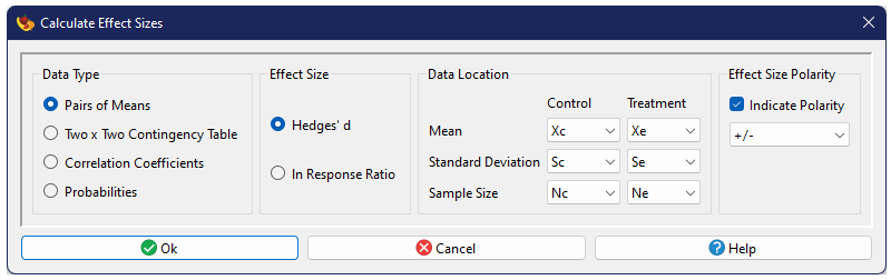
The effect size calculation dialog has four sections: (1) specification of data type, (2) specification of effect size metric, (3) specification of data sources, and (4) an optional specification of effect size polarity. Three data types are currently supported, each with its own set of effect size metrics and data requirements, described below.
Effect size polarity should be used to standardize the sign (polarity) of the effect size metrics, when not all experimental conditions were conducted in the same direction. As an example, if some studies were based on the addition of CO2 to a system while others were based on the removal of CO2 from a system, the expectation is that a positive effect for one would be equivalent to a negative for the other. The polarity indicator lets a user specify which studies were measured in the same "direction" and will automatically reverse signs of those in the opposite so that all calculated effect sizes represent the same thing.
The polarity columns can contain numbers or text. Generally one would use a simple indicator, such as the numbers 1 and -1 or the symbols + and -. The actual programatic interpretation, is that if the value is a number, negative values are used to indicate negative polarity, while positive values and zero indicate positive polarity. If the value is not a number, a negative sign "-" indicates negative polarity, while any other value indicates positive polarity.
will attempt to calculate effect sizes for all rows in the data matrix, whether filtering has been enabled or not. Rows for which an effect size cannot be calculated, whether because of missing data or invalid values, will be left blank in the resulting columns in the data table and will be indicated in the text output.
Effect Size Calculation Output
When effect sizes are calculated, two new columns are added to the data matrix, one containing the effect size for each study and one the estimated variance of that effect size. Rows containing missing or invalid data for the effect size chosen will remain blank. In addition, the data options and the values are reported in the Output Tab, as in this example of output:
Calculate Effect Sizesln Response Ratio
→ Citation: Hedges et al. (1999)Data obtained from columns:
→ Control Means: Xc
→ Control Sample Sizes: Nc
→ Control Standard Deviations: Sc
→ Treatment Means: Xe
→ Treatment Sample Sizes: Ne
→ Treatment Standard Deviations: Se
→ Effect Size Polarity Indicator: +/-ReferencesStudy ln Response Ratio var(ln Response Ratio) --------------------------------------------------- Row 1 0.0199 0.0758 Row 2 0.3211 0.0515 Row 3 -0.1542 0.0214 Row 4 -0.2412 0.0072 Row 5 -0.3567 0.0067 Row 6 -0.6022 0.0217 Row 7 1.2088 0.7026 Row 8 No effect size could be calculated Row 9 No effect size could be calculated Row 10 No effect size could be calculated Row 11 0.0000 0.0599 Row 12 -0.2392 0.0225 Row 13 1.1399 0.1608 Row 14 No effect size could be calculated Row 15 No effect size could be calculated Row 16 1.5072 0.4254 Row 17 No effect size could be calculated Row 18 No effect size could be calculated Row 19 1.3030 0.2828 Row 20 No effect size could be calculated Row 21 No effect size could be calculated Row 22 0.3045 0.0161 Row 23 3.1676 4.5598 Row 24 No effect size could be calculated Row 25 No effect size could be calculated Row 26 No effect size could be calculated Row 27 0.1341 0.0135 Row 28 0.2351 0.4182 Row 29 No effect size could be calculated Row 30 1.6285 0.4528 Row 31 No effect size could be calculated Row 32 -0.4783 0.4762 Row 33 No effect size could be calculated Row 34 No effect size could be calculated Row 35 1.4748 2.0064 Row 36 1.7636 3.4144 Row 37 No effect size could be calculated Row 38 No effect size could be calculated Row 39 No effect size could be calculated Row 40 -0.6931 1.1990 Row 41 0.5613 0.1377 Row 42 -0.6870 0.0613 Row 43 -0.2818 0.1472Hedges, L.V., J. Gurevitch, and P.S. Curtis (1999) The meta-analysis of response ratios in experimental ecology. Ecology 80(4):1150–1156.
Pairs of Means
One common type of data comes from studies which compare two estimated means (\(\bar{y}_1\) and \(\bar{y}_2\)), along with associated sample sizes (\(n_1\) and \(n_2\)) and standard deviations (\(s_1\) and \(s_2\)). The common effect sizes calculated from pairs of means are based on their standardized difference or their ratio.
Hedges' d
Many estimates of a standardized difference of means have been proposed for meta-analysis, but the most widely used and preferred metric is generally known as Hedges' d (Hedges and Olkin 1985). It is calculated as
$$d=\frac{\bar{y}_1 - \bar{y}_2}{\sqrt{\frac{\left(n_1 - 1\right)s^{2}_i + \left(n_2 - 1\right)s^{2}_2}{n_1 + n_2 - 2}}}J,$$
where
$$J=1-\frac{3}{4\left(n_1 + n_2 - 2\right) - 1}$$
is a correction for small sample size. Hedges' d has an associaed variance estimate of
$$v_d=\frac{n_1 + n_2}{n_1 n_2} + \frac{d^2}{2\left(n_1 + n_2\right)}.$$
ln Response Ratio
An alternate effect size to the standardized mean difference is the ratio of the means, also known as the response ratio (Hedges et al. 1999). It is useful when one wishes to compare the magnitudes of two means with the same sign. However, as ratios generally have poor statistical properties, one instead transforms the ratio to a metric with more desirable properties using the natural log. The natural log of the response ratio is calculated as
$$\ln{R}=\ln{\frac{\bar{y}_1}{\bar{y}_2}},$$
with variance
$$v_{\ln{R}}=\frac{s_1^2}{n_1 \bar{y}_1^2} + \frac{s_2^2}{n_2 \bar{y}_2^2}.$$
Two × Two Contingency Table
A common form of contrasting data in medical research and related fields is a contingency table. This compares two groups (generally, a treatment and a control) and the observed counts (A, B, C, and D in the following table) for two possible outcomes (frequently a positive and a negative outcome, e.g., alive vs. dead).
| Control | Treatment | Total | |
|---|---|---|---|
| Response | \(A\) | \(B\) | \(A+B\) |
| No Response | \(C\) | \(D\) | \(C+D\) |
| Total | \(n_1 = A+C\) | \(n_2 = B+D\) | \(A+B+C+D\) |
Before effect sizes can be calculated for this sort of data, one must generally first determine the rate of response for each group. The rate ranges from zero to one, and can be interpreted as the probability of a member of that group showing the response. The rate \(P\) is simply the number that show the response divided by the total, or
$$P_1 = \frac{A}{n_1}\text{, }P_2 = \frac{B}{n_2}.$$
From these there are three common effect size measures.
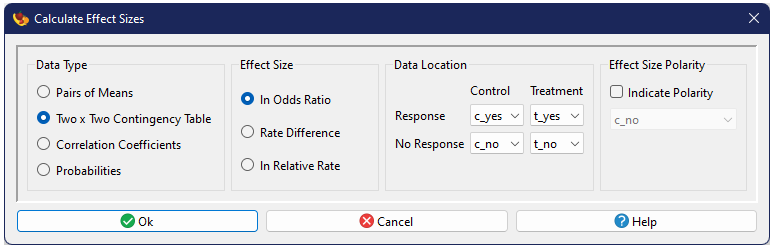
ln Odds Ratio
While there are a number of simple ways to calculate the odds ratio and its variance, but for the purposes of meta-analysis there is a more complicated approach (Mantel and Haenzel 1959) that gives better statistical results, particularly when sample sizes are small. In this approach the observed response from the first (control) group is simply
$$O = A.$$
The expected response for this group if there were no differences between the two groups is
$$\hat{O} = \frac{\left(A+B\right)\left(A+C\right)}{\left(A+B+C+D\right)}.$$
The variance of the difference between these two values is
$$V = \hat{O}\left(\frac{A+C}{A+B+C+D}\right) \left(\frac{C+D}{A+B+C+D-1}\right).$$
These allow the ln odds ratio to be estimated as
$$\ln OR = \frac{O - \hat{O}}{V},$$
with variance
$$v_{\ln OR} = \frac{1}{V}.$$
Rate Difference
The rate difference (DerSimonian and Laird 1986, L’Abbé et al. 1987, Berlin et al. 1989, Normand 1999) is simply the difference in rates, or
$$RD = P_1 - P_2,$$
with variance
$$v_{RD} = \frac{P_1 \left(1-P_1\right)}{n_1} + \frac{P_2 \left(1-P_2\right)}{n_2}.$$
ln Relative Rate
The relative rate (or rate ratio) (Greenland 1987, L’Abbé et al. 1987, Normand 1999) is generally log-transformed as
$$\ln RR = \ln\frac{P_1}{P_2}$$
with variance
$$v_{\ln RR} = \frac{1 - P_1}{n_1 P_1} + \frac{1 - P_2}{n_2 P_2}.$$
Correlation Coefficients
When association between two continuous variables is of interest, Pearson's correlation coefficient r, combined with its sample size, is commonly used as an effect-size measure.
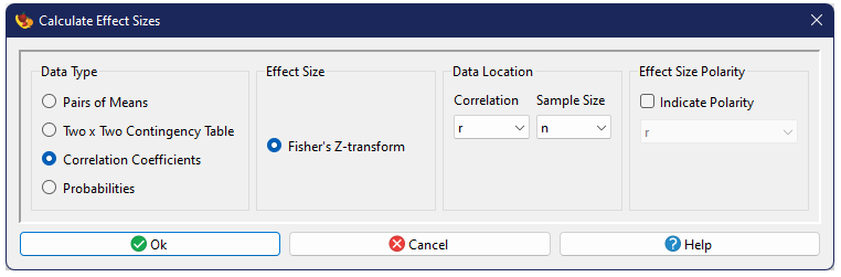
Fisher's Z-transform
Because the distribution of Pearson's correlation is skewed as it approaches ±1, it is generally first transformed using Fisher's Z-transformation (Fisher 1928):
$$z=\frac{1}{2}\ln\left(\frac{1+r}{1-r} \right),$$
whose asymptotic variance estimate (Sokal and Rohlf 1995) is simply
$$v_z=\frac{1}{n-3}.$$
Probabilities
When probabilities are available, combined with their sample size, one can use the logit as an effect size measure (Mengersen and Gurevitch 2013).
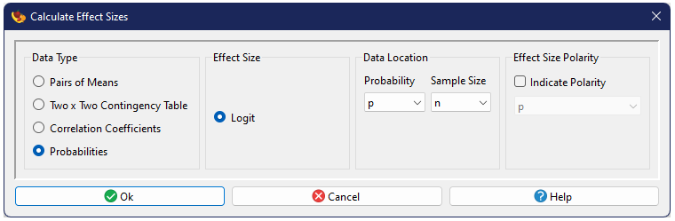
Logit
The logit is essentially the log-odds, and is calculated as
$$\text{logit}=\ln\left(\frac{p}{1-p}\right),$$
with variance
$$v_{\text{logit}}=\sqrt{\frac{1}{np} + \frac{1}{n\left(1-p\right)}}.$$
Publication Bias
Publication bias analysis can be accessed by choosing
from the
menu or
 from the toolbar. Doing
so will bring up a dialog where you can choose the type of analysis you want to perform.
from the toolbar. Doing
so will bring up a dialog where you can choose the type of analysis you want to perform.
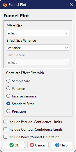
Funnel Plot
A funnel plot is a special type of scatter plot where a metric (in meta-analysis, usually an effect size) is plotted against sample size or an estimate of variance (Light and Pillemer 1984). The idea of a funnel plot is that if there is a single true value being estimated from all of the studies, those with high variance (or low sample size) will tend to vary a lot around the true value, while those with low variance (or high sample size) will tend to vary only a little around the true value. With a large number of studies you would expect the scatter to be funnel-shaped and symmetric around the true value. If the funnel is asymmetric, this may be an indication of publication bias.
If plotting effects size against variance or a derivative (rather than sample size), it is possible to various forms of confidence intervals or power information around the funnel, based on the standard error and a Normal distribution. Options include:
- pseudo-confidence interval (Sterne and Egger 2001), which creates a 95% envelope around the mean effect size (under a fixed-effects model)
- contour confidence intervals (Peters et al. 2008), which create zones of statistical significance (<90%, 90-95%, 95-99%, >99%) around a null effect size of zero
- power-enhancement (sunset) plot (Kossmeier et al. 2020) which uses color shading of the background to indicate the power of a particular study to indicate a significant effect of interest
Drawing a Funnel Plot
Funnel Plot creation is found as part of the /
analyses. In
these figures, the effect size will be plotted on the x-axis, with five options for the y-axis:
(1) sample size, (2) variance, (3) inverse variance (=weight), (4) standard error (the square-root
of variance in this formulation), and (5) precision (1/SE). All options require specification of
effect size and variance data (in order to calcualte the mean effect). The first also requires
one to specify sample size. When variance or standard error is chosen as an option, the
y-axis is automatically reversed (smallest numbers at top of axis rather than bottom) so that the
expected funnel direction will be consistent across all choices (i.e., widest at the bottom
of the figure, narrowest at the top).
In addition to the scattered points, the plot will include a vertical line for the mean effect size (assuming a simple weighted, fixed-effects model). For options other than sample size, one can also choose to plot the 95% pseudo-confidence interval, the contour confidence intervals, and/or the power-enhancement (sunset) background colors.
These methods are intrinsically graphical, so always produces a figure and the related text output is fairly minimal.
Output Examples
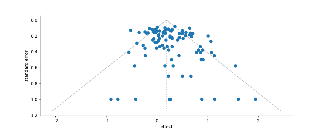
Funnel plot of effect vs. standard error. The dotted silver line represents the mean effect size. The dashed silver line represents the 95% pseudo-confidence interval of the funnel, after Sterne and Egger (2001).
References
Light, R.J., and D.B. Pillemer (1984) Summing Up: The Science of Reviewing Research. Harvard University Press: Cambridge.
Sterne, J.A.C., and M. Egger (2001) Funnel plots for detecting bias in meta-analysis: Guidelines on choice of axis. Journal of Clinical Epidemiology 54(10):1045–1055. DOI: 10.1016/S0895-4356(01)00377-8
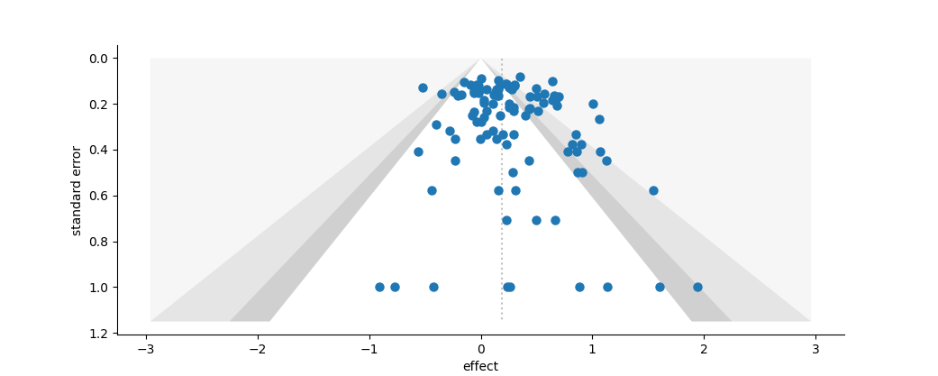
Funnel plot of effect vs. standard error. The dotted silver line represents the mean effect size. The very light pink zone represents the area where effect sizes would have a probability of less than 1%, the silver zone a probability between 1 and 5%, and the cool grey zone a probability between 5 and 10%, after Peters et al. (2008).
References
Light, R.J., and D.B. Pillemer (1984) Summing Up: The Science of Reviewing Research. Harvard University Press: Cambridge.
Peters, J.L., A.J. Sutton, D.R. Jones, K.R. Abrams, and L. Rushton (2008) Contour-enhanced meta-analysis funnel plots help distinguish publication bias from other causes of asymmetry. Journal of Clinical Epidemiology 61(10):991–996. DOI: 10.1016/j.jclinepi.2007.11.010
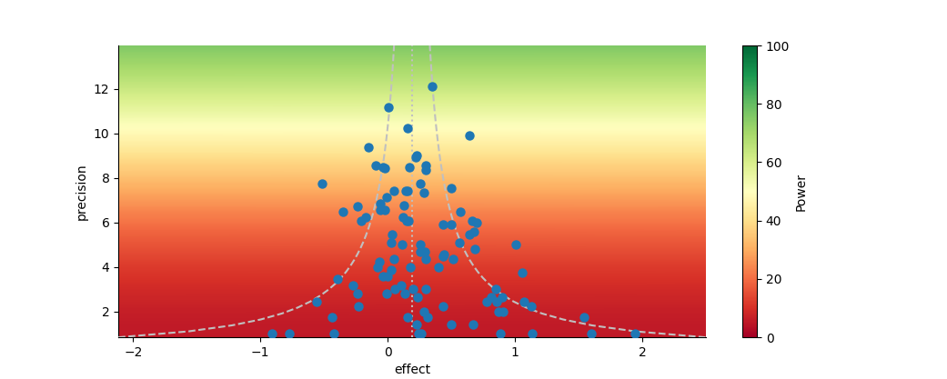
Funnel plot of effect vs. precision. The dotted silver line represents the mean effect size. The dashed silver line represents the 95% pseudo-confidence interval of the funnel, after Sterne and Egger (2001). The background colors indicate the power of an individual study to detect an underlying true effect equal to the mean, after Kossmeier et al. (2020).
References
Kossmeier, M., U.S. Tran, and M. Voracek (2020) Power-enhanced funnel plots for meta-analysis: The sunset funnel plot. Zeitschrift für Psychologie 228(1):43–49. DOI: 10.1027/2151-2604/a000392
Light, R.J., and D.B. Pillemer (1984) Summing Up: The Science of Reviewing Research. Harvard University Press: Cambridge.
Sterne, J.A.C., and M. Egger (2001) Funnel plots for detecting bias in meta-analysis: Guidelines on choice of axis. Journal of Clinical Epidemiology 54(10):1045–1055. DOI: 10.1016/S0895-4356(01)00377-8
Egger Regression
Egger Regression (Egger et al. 1997) is a simple analysis designed to formally test for the symmetry desired from a funnel plot. In this test one performs a simple linear regression of a standardized effect size (the effect size × precision) against the precision (the square-root of the variance). Unlike most linear regressions, the focus of this test is on the intercept rather than the slope: In an unbiased, symmetric data set the intercept is expected to be zero. If the intercept is not zero, the data is thought to deviate from this symmetric expectation.
The structure of this test is almost identical to the regression from a Galbraith (Radial) Plot, except in that plot the slope is forced through the origin while the Egger test actually examines if it goes through the origin on its own.
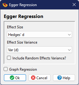
Running an Egger Regression
The Egger Regression only uses a single dialog where you can specify the data sources, whether you want the analysis performed assuming a fixed (default) or random-effects model, and whether you want the resulting regression graphed. The results are simply a table with the intercept and slope of the regression, their standard errors, confidence intervals and significance (based on Student's t-distribution).
Output
The following is an example of the output from an Egger Regression.
Publication Bias
Egger Regression
→ Citations: Egger et al. (1997)
→ Random Effects Model→ Effect Sizes: Hedges' d
→ Effect Size Variances: Var (d)25 studies will be included in this analysis
Predictor    Value      SE     df        95% CI          P(t)
--------------------------------------------------------------
Intercept   -0.0236   1.0387   23   -2.1723 to 2.1251   0.9821
Slope        0.3385   0.3468   23   -0.3789 to 1.0560   0.3392
References
Egger, M., G.D. Smith, M. Schneider, and C. Minder (1997) Bias in meta-analysis detected by a simple, graphical test. BMJ 315:629–634. DOI: 10.1136/bmj.315.7109.629
Lin, L., and H. Chu (2018) Quantifying publication bias in meta-analysis. Biometrics 74(3):785–794. DOI: 10.1111/biom.12817
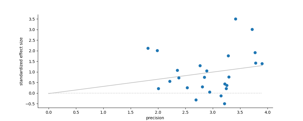
Plot of standardized effect size vs. precision, under a random effects model.
Rank Correlation Analysis
Rank Correlation Analysis (Begg 1994; Begg and Mazumdar 1994) is a simple test for publication bias, which uses a correlation of ranks to look for a relationship between a standardized effect size and either sample size or a standardized variance. The test is considered a statistical analogue of a funnel plot. For each study, the standardized variance is calculated as:
$$v_i^* = v_i - 1/{\sum{w}} ,$$
and the standardized effect size of each study is calculated as
$$\theta_i^* = \frac{\theta_i - \bar{\theta}}{\sqrt{v_i^*}}.$$
This standardized effect size is then compared to either the individual study sample sizes or the standardized variance using a rank correlation test (Sokal and Rohlf 1995). A significant correlation may indicate a publication bias where larger effect sizes (in one direction, e.g., positive) are more likely to be published than smaller ones.
Running a Rank Correlation Analysis
The Rank Correlation Analysis only uses a single dialog. Other than choosing the data sources, the dialog asks whether the user wants the correlation to be vs. standardized variance or sample size, where the latter choice then also requires the user to input the column containing sample sizes.
Additionally, there is an option to perform the rank correlation using Kendall's τ (Kendall 1938) or Spearman's ρ (Spearman 1904). Because the distribution of these metrics can be complicated, particularly when the number of studies is low, automatically uses a randomization procedure to thest their significance, with the number of iterations user-specifiable.
Output
The following is an example of the output from a Rank Correlation Analysis.
Analysis
Rank Correlation Analysis
→ Citations: Begg (1994), Begg and Mazumdar (1994)→ Effect Sizes: effect
→ Effect Size Variances: variance
→ Rank Correlation Method: Kendall's τ
→ Citation: Kendall (1938)
→ Fixed Effects Model→ Randomization to test correlation: 999 iterations
85 studies will be included in this analysis
Rank Correlation Results
Kendall's τ = 0.2826
Probability = 0.0010References
Begg, C.B. (1994) Publication bias. Pp. 399-409 in The Handbook of Research Synthesis, H. Cooper and L.V. Hedges, eds. Sage, New York.
Begg, C.B., and M. Mazumdar (1994) Operating characteristics of a rank correlation test for publication bias. Biometrics 50:1088–1101.
Kendall, M. (1938) A new measure of rank correlation. Biometrika. 30(1–2):81–89.
Sokal, R.R., and F.J. Rohlf (1995) Biometry (3rd edition). Freeman, San Francisco.
Trim and Fill Analysis
"Trim and Fill" is a simple method to adjust for funnel plot asymmetry. It analyzes the distribution of points and estimates "missing" studies in order to create the expected symmetry of an unbiased funnel plot (Duval and Tweedie 2000a, 2000b).
Fundamentally the analysis works by iteratively estimating the asymmetry of the data around the mean, and then removing a number of studies until symmetry is achieved. At this point the removed studies are added back into the dataset, along with imputed "missing" studies that are the mirror image (reflected across the mean) of those same re-added studies. The mean (and median) pre- and post-addition of the imputed studies are reported.
Three different estimators of the number of missing studies are described by Duval and Tweedie (2000a), all of which are options within .
Running a Trim and Fill analysis
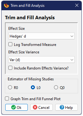
The Trim and Fill analysis only uses a single dialog. Other than choosing the data sources and whether you want a graph of the results, the one additional option is which of the three estimators you wish to use for the analysis: R0, L0, or Q0.
Output
The following is an example of the output from a trim and fill analysis. It includes the estimated number of missing studies and the mean and median before and after imputation of these missing studies.
Analysis
Trim and Fill Analysis
→ Citations: Duval and Tweedie (2000a), Duval and Tweedie (2000b)→ Effect Sizes: effect
→ Effect Size Variances: variance
→ Estimator of Missing Studies: L0
→ Fixed Effects Model→ Standard confidence intervals around means based on Normal distribution
85 studies will be included in this analysis
Trim and Fill Analysis estimated 19 missing studies.
Mean Effect Sizesn Mean Median 95% CI -------------------------------------------------------------------- Original Mean effect 85 5.0777 4.9119 4.9019 to 5.2534 Trim and Fill Mean effect 104 4.9453 4.8298 4.7747 to 5.1159References
Duval, S. and R. Tweedie (2000a) A nonparametric "trim and fill" method of accounting for publication bias in meta-analysis. Journal of the American Statistical Association 95(449):89–98.
Duval, S. and R. Tweedie (2000b) Trim and fill: A simple funnel-plot-based method of testing and adjusting for publication bias in meta-analysis. Biometrics 56:455–463.
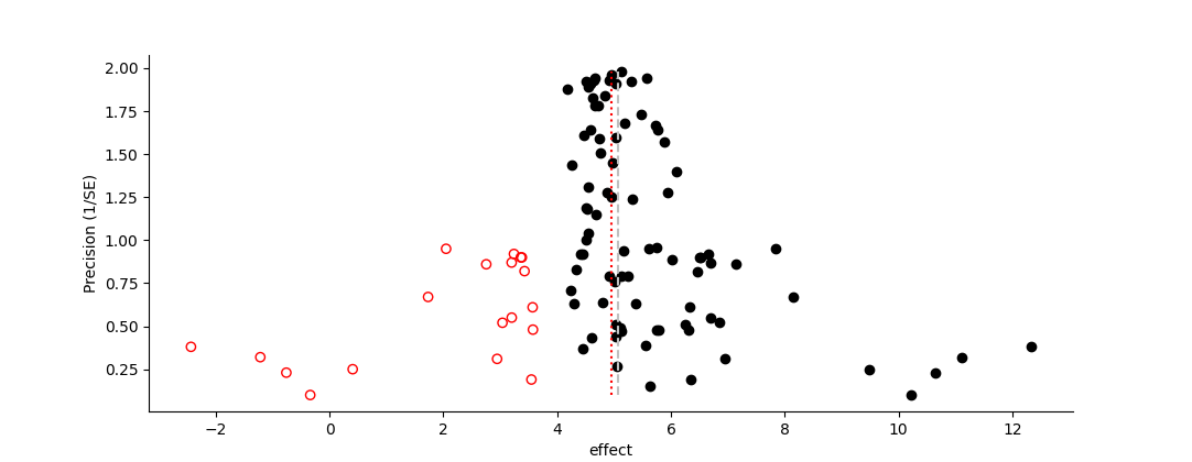
Funnel plot of effect vs. precision, showing the results of a Trim and Fill Analysis (Duval and Tweedie 2000a, b). Solid black circles represent the original data; open red circles represent inferred "missing" data. The dashed line represents the mean effect size of the original data, the dotted line the mean effect size including the inferred data.References
Duval, S. and R. Tweedie (2000a) A nonparametric "trim and fill" method of accounting for publication bias in meta-analysis. Journal of the American Statistical Association 95(449):89–98.
Duval, S. and R. Tweedie (2000b) Trim and fill: A simple funnel-plot-based method of testing and adjusting for publication bias in meta-analysis. Biometrics 56:455–463.
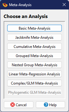
Analyses
All primary meta-analysis computation can be accessed by choosing
from the
menu or
 from the toolbar. Doing so
will bring up a dialog where you can choose the type of analysis you want to perform. The
Phylogenetic GLM Meta-Analysis option will only be enabled if you have already
loaded a phylogeny into memory.
from the toolbar. Doing so
will bring up a dialog where you can choose the type of analysis you want to perform. The
Phylogenetic GLM Meta-Analysis option will only be enabled if you have already
loaded a phylogeny into memory.
Choosing a particular analysis will bring up two (in most cases) additional dialogs where the user can specify data inputs and options for that particular analysis type.
Remember that any studies that have been marked for filtering will automatically be excluded from these analyses. Any filtered studies will be listed at the top of the output, as well as any studies which could not be included due to missing or invalid data.
Common Options
Options common to all or most of the analyses will be described here, with specifics on each analysis described in their own section below.
Effect Size and Variance
All analyses require the user to specify an effect size and its associated variance. If the effect size was calculated within , it will set that value (and its variance) as the default choices, although users can choose another. The program will also remember the last choices from previous analyses.
In the equations in the following sections, the effect size from the ith study will be indicated as \(\theta_i\), its associated variance as \(v_i\), and its associated weight \(w_i = 1/v_i\). The total number of studies included in the analysis is \(n\).
Most analyses also have a checkbox titled Log Transformed Measure. If the effect size was calculated by , it will automaticaly check this box if that effect size is chosen for the analysis, although the user can uncheck it. The user can also choose this option for an imported effect size. It is important to note that whether the box is checked or not does not change the primary analysis in any manner. If the box is checked, additional output will be provided reporting mean effect sizes (and confidence intervals) as exponentiated ("de-logged") values. The log transformed values will still be reported as normal.
Random Effects Variance
Most analyses include a checkbox for specifying random effects variance. By default, analyses will be conducted in a fixed-effects model framework. Checking this box will conduct the analysis in a random-effects model framework (for some types of analyses, alternative referred to as a mixed-effects model).
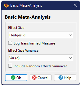
Basic Meta-Analysis
The basic meta-analysis option represents a "classic" meta-analysis where all studies are being combined into a single (global) mean value. This is a weighted mean, calculated as
$$\bar{\theta} = \frac{\sum{w_i \theta_i}}{\sum{w_i}},$$
with variance
$$s_{\bar{\theta}}^2 = \frac{1}{\sum{w_i}},$$
and a confidence interval determined through a normal distribution or a bootstrap procedure, if desired. The total heterogeneity statistic is determined as
$$Q_T = \sum{w_i\left(\theta_i - \bar{\theta}\right)^2},$$
which can be tested against a χ2 distribution with \(n-1\) degrees of freedom.
\(I^2\), an alternative to Q-statistics (Higgins and Thompson 2002) is calculated as
$$I^2 = \max \left[{0, 100 \times \frac{Q_T - \left(n - 1\right)}{Q_T}}\right],$$
with its confidence interval determined through the methods of Higgins and Thompson (2002) and Huedo-Medina et al. (2006). An estimate of pooled variance is determined as
$$\hat{\sigma}^2 = \frac{Q_T - (n - 1)}{\sum{w_i} - \frac{\sum{w_i^2}}{\sum{w_i}}}.$$
For a random-effects model, the weights are recalculated as
$$w_i^* = 1/{\left(v_i + \hat{\sigma}^2\right)} ,$$
and the rest of the calculations repeated using these new weights.
Running a basic analysis
The basic options are just specification of the effect size and variance and whether one wishes to implement a random-effects model (rather than the fixed-effects default).
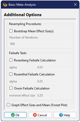
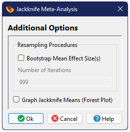
The second dialog includes a number of additional options.
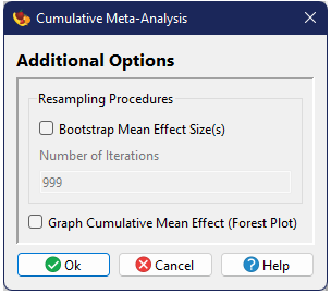
Resampling procedures
One can optionally conduct a bootstrap procedure in order to estimate confidence intervals around the mean (Adams et al. 1997). The number of iterations for the bootstrap can also be specified.
Failsafe Tests
Failsafe tests can be conducted using three different methods, that of Rosenthal (1979), Orwin (1983), and Rosenberg(2005). For each method you can specify the desired threshold. (Note: for Orwin's method, if you enter a negative threshold, the method assumes you are looking for a minimal negative effect rather than a minimum positive effect). Failesafe tests are only included as an option of the basic analysis because the logic of the failsafe estimate only applies to this simple model.
Graphical Output
One can optionally include a graphical figure as output. For this analysis this will be a forest plota>, showing the global mean and its confidence intervals at the top of the figure, with all of the individual studies beneath.
Output
The following is an example of the output from a basic analysis. Specifics are dependent on the options chosen as well as the data.
AnalysisStructure: None → Citation: Hedges and Olkin (1985)
→ Effect Sizes: Hedges' d
→ Effect Size Variances: Var (d)
→ Fixed Effects Model→ Standard confidence intervals around means based on Normal distribution
→ Use bootstrap for confidence intervals around means: 999 iterations
→ Citations: Adams et al. (1997), Dixon (1993)25 studies will be included in this analysis
Heterogeneity
Source      Q      df   P(χ2)
------------------------------
Total    46.5517   24   0.0038
→ Citation: Hedges and Olkin (1985)
Source     I2            95% CI
-------------------------------------
Total    48.4444   17.9350 to 67.6113
→ Citations: Higgins and Thompson (2002), Huedo-Medina et al. (2006)
Mean Effect Size
   n     Mean    Median        95% CI          Bootstrap CI     Bias-corrected CI
---------------------------------------------------------------------------------
   25   0.3588   0.3585   0.2706 to 0.4470   0.2161 to 0.4887    0.2310 to 0.4980
Sqrt Pooled Variance = 0.2205
Mean Study Variance = 0.0838
ratio = 2.6309Rosenberg's Fail-safe Number
→ Citation: Rosenberg (2005)
→ alpha: 0.0500Fail-safe n (normal distribution) = 388.8247
Fail-safe n (t distribution, 1 study of n × avg weight) = 349.7769
Fail-safe n (t distribution, n studies of avg weight) = 386.3860Rosenthal's Fail-safe Number
→ Citation: Rosenthal (1979)
→ alpha: 0.0500Fail-safe n = 302.6107
Orwin's Fail-safe Number
→ Citation: Orwin (1983)
→ Minimal Effect Size: 0.2000Fail-safe n = 19.8523
References
Adams, D.C., J. Gurevitch, and M.S. Rosenberg (1997) Resampling tests for meta-analysis of ecological data. Ecology 78:1277–1283.
Dixon, P.M. (1993) The bootstrap and the jackknife: Describing the precision of ecological indices. Pp. 290—318 in Design and Analysis of Ecological Experiments, S.M. Scheiner and J. Gurevitch, eds. Chapman and Hall, New York.
Hedges, L.V. and I. Olkin (1985) Statistical Methods for Meta-analysis. Academic Press, Orlando, FL.
Higgins, J.P.T. and S.G. Thompson (2002) Quantifying heterogeneity in a meta-analysis. Statistics in Medicine 21:1539–1558.
Huedo-Medina, T.B., J. Sánchez-Meca, F. Marín-Martínez, and J. Botella (2006) Assessing heterogeneity in meta-analysis: Q statistic or I2 index? Psychological Methods 11:193–206.
Orwin, R.G. (1983) A fail-safe N for effect size in meta-analysis. Journal of Educational Statistics 8(2):157–159.
Rosenberg, M.S. (2005) The file-drawer problem revisited: A general weighted method for calculating fail-safe numbers in meta-analysis. Evolution 59(2):464–468.
Rosenthal, R. (1979) The “file drawer problem” and tolerance for null results. Psychological Bulletin 86(3):638–641.
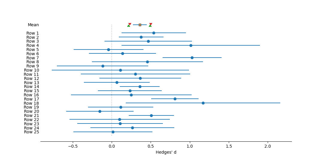
Forest plot of individual effect sizes for each study, as well as the overall mean. Effect size measured as Hedges' d. The dotted vertical line represents no effect, or a mean of zero. Circles represent mean effect size, with the corresponding line the 95% confidence interval. X's represent the median. Upward-pointing triangles mark the confidence interval from a bootstrap (999 iterations) procedure, following Adams et al. (1997); downward-pointing triangles mark the bias-corrected bootstrap interval.References
Adams, D.C., J. Gurevitch, and M.S. Rosenberg (1997) Resampling tests for meta-analysis of ecological data. Ecology 78:1277–1283.
Jackknife Meta-Analysis
Jacknnife Meta-Analysis (also known as Leave-one-out Meta-analysis) is a statistical procedure for examining the effects of individual studies on the global mean. The full analysis is run with a single study left out, systematically repeating the procedure across all possible studies. This is a form of sensitivity analysis to potentially identify outliers and allows one to judge whether the overall results are being skewed by a single study.
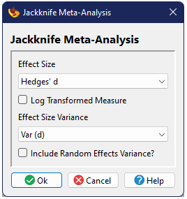
Running a Jackknife analysis
The options for a Jackknife Meta-Analysis are essentially identical to the Basic Analysis, except that the Failsafe Number tests are not included.
Output
The output for a Jacknife Meta-Analysis is similar to that from a Basic Analysis, except with the addition of tables illustrating the heterogenity and means for each case of a study being excluded from the analysis. The other difference is in the graphical output, if requested. In a Basic Analysis, the forest plot illustrates the global mean as well as the individual effect size for each study. In the Jackknife analysis the plot illustrates the global mean, as well as the estimated mean when each study is excluded from the analysis.
AnalysisJackknife Meta-Analysis
→ Effect Sizes: Hedges' d
→ Effect Size Variances: Var (d)
→ Fixed Effects Model→ Standard confidence intervals around means based on Normal distribution
→ Use bootstrap for confidence intervals around means: 999 iterations
→ Citations: Adams et al. (1997), Dixon (1993)25 studies will be included in this analysis
Jackknife Results
Heterogeneity
     Source            Q      df   P(χ2)
-----------------------------------------
w/o Row 1 Qtotal    45.7844   23   0.0032
w/o Row 2 Qtotal    46.5360   23   0.0026
w/o Row 3 Qtotal    46.4003   23   0.0027
w/o Row 4 Qtotal    44.4476   23   0.0046
w/o Row 5 Qtotal    43.3642   23   0.0063
w/o Row 6 Qtotal    45.4801   23   0.0035
w/o Row 7 Qtotal    33.8172   23   0.0678
w/o Row 8 Qtotal    46.4768   23   0.0026
w/o Row 9 Qtotal    43.9570   23   0.0053
w/o Row 10 Qtotal   46.2407   23   0.0028
w/o Row 11 Qtotal   46.5282   23   0.0026
w/o Row 12 Qtotal   46.5510   23   0.0026
w/o Row 13 Qtotal   44.6085   23   0.0044
w/o Row 14 Qtotal   46.5517   23   0.0026
w/o Row 15 Qtotal   46.1621   23   0.0029
w/o Row 16 Qtotal   46.4752   23   0.0026
w/o Row 17 Qtotal   37.2017   23   0.0310
w/o Row 18 Qtotal   43.9570   23   0.0053
w/o Row 19 Qtotal   45.1825   23   0.0038
w/o Row 20 Qtotal   40.8919   23   0.0122
w/o Row 21 Qtotal   45.4327   23   0.0035
w/o Row 22 Qtotal   45.9154   23   0.0031
w/o Row 23 Qtotal   45.7182   23   0.0032
w/o Row 24 Qtotal   46.4262   23   0.0026
w/o Row 25 Qtotal   44.7292   23   0.0043
Mean Effect Sizes
                       n     Mean    Median        95% CI          Bootstrap CI     Bias-corrected CI
-----------------------------------------------------------------------------------------------------
w/o Row 1 Hedges' d    24   0.3502   0.3585   0.2599 to 0.4405   0.2039 to 0.4895    0.2164 to 0.4979
w/o Row 2 Hedges' d    24   0.3570   0.3585   0.2643 to 0.4497   0.2101 to 0.5066    0.2218 to 0.5138
w/o Row 3 Hedges' d    24   0.3560   0.3585   0.2667 to 0.4453   0.2158 to 0.4835    0.2260 to 0.4952
w/o Row 4 Hedges' d    24   0.3523   0.3585   0.2637 to 0.4409   0.2070 to 0.4836    0.2070 to 0.4840
w/o Row 5 Hedges' d    24   0.3750   0.3585   0.2850 to 0.4649   0.2400 to 0.5079    0.2499 to 0.5143
w/o Row 6 Hedges' d    24   0.3686   0.3585   0.2785 to 0.4587   0.2248 to 0.5006    0.2366 to 0.5128
w/o Row 7 Hedges' d    24   0.3203   0.3585   0.2296 to 0.4110   0.1899 to 0.4347    0.2008 to 0.4407
w/o Row 8 Hedges' d    24   0.3573   0.3585   0.2684 to 0.4462   0.2178 to 0.4968    0.2178 to 0.5004
w/o Row 9 Hedges' d    24   0.3698   0.3585   0.2806 to 0.4591   0.2381 to 0.5196    0.2468 to 0.5266
w/o Row 10 Hedges' d   24   0.3614   0.3585   0.2727 to 0.4500   0.2191 to 0.4940    0.2294 to 0.5005
w/o Row 11 Hedges' d   24   0.3597   0.3585   0.2708 to 0.4486   0.2098 to 0.4936    0.2099 to 0.4947
w/o Row 12 Hedges' d   24   0.3586   0.3585   0.2691 to 0.4481   0.2222 to 0.4913    0.2252 to 0.5020
w/o Row 13 Hedges' d   24   0.3722   0.3585   0.2820 to 0.4624   0.2212 to 0.5058    0.2266 to 0.5130
w/o Row 14 Hedges' d   24   0.3589   0.3656   0.2649 to 0.4528   0.2026 to 0.5083    0.2158 to 0.5218
w/o Row 15 Hedges' d   24   0.3650   0.3585   0.2747 to 0.4553   0.2296 to 0.5088    0.2354 to 0.5186
w/o Row 16 Hedges' d   24   0.3603   0.3585   0.2715 to 0.4490   0.2187 to 0.4979    0.2227 to 0.4991
w/o Row 17 Hedges' d   24   0.3168   0.3585   0.2245 to 0.4090   0.1904 to 0.4472    0.1980 to 0.4533
w/o Row 18 Hedges' d   24   0.3523   0.3585   0.2638 to 0.4409   0.2107 to 0.4864    0.2123 to 0.4874
w/o Row 19 Hedges' d   24   0.3701   0.3585   0.2799 to 0.4604   0.2256 to 0.5104    0.2336 to 0.5255
w/o Row 20 Hedges' d   24   0.3812   0.3585   0.2911 to 0.4713   0.2470 to 0.5163    0.2574 to 0.5224
w/o Row 21 Hedges' d   24   0.3435   0.3585   0.2509 to 0.4362   0.1967 to 0.4847    0.2102 to 0.4971
w/o Row 22 Hedges' d   24   0.3638   0.3585   0.2748 to 0.4528   0.2281 to 0.4996    0.2305 to 0.5075
w/o Row 23 Hedges' d   24   0.3655   0.3585   0.2762 to 0.4549   0.2263 to 0.5105    0.2323 to 0.5120
w/o Row 24 Hedges' d   24   0.3615   0.3585   0.2721 to 0.4509   0.2198 to 0.4880    0.2230 to 0.4883
w/o Row 25 Hedges' d   24   0.3696   0.3585   0.2800 to 0.4591   0.2405 to 0.5156    0.2406 to 0.5198
Global Results
Heterogeneity
Source      Q      df   P(χ2)
------------------------------
Total    46.5517   24   0.0038
→ Citation: Hedges and Olkin (1985)
Source     I2            95% CI
-------------------------------------
Total    48.4444   17.9350 to 67.6113
→ Citations: Higgins and Thompson (2002), Huedo-Medina et al. (2006)
Mean Effect Size
   n     Mean    Median        95% CI          Bootstrap CI     Bias-corrected CI
---------------------------------------------------------------------------------
   25   0.3588   0.3585   0.2706 to 0.4470   0.2156 to 0.4898    0.2309 to 0.5003
Sqrt Pooled Variance = 0.2201
Mean Study Variance = 0.0838
ratio = 2.6266References
Adams, D.C., J. Gurevitch, and M.S. Rosenberg (1997) Resampling tests for meta-analysis of ecological data. Ecology 78:1277–1283.
Dixon, P.M. (1993) The bootstrap and the jackknife: Describing the precision of ecological indices. Pp. 290—318 in Design and Analysis of Ecological Experiments, S.M. Scheiner and J. Gurevitch, eds. Chapman and Hall, New York.
Hedges, L.V. and I. Olkin (1985) Statistical Methods for Meta-analysis. Academic Press, Orlando, FL.
Higgins, J.P.T. and S.G. Thompson (2002) Quantifying heterogeneity in a meta-analysis. Statistics in Medicine 21:1539–1558.
Huedo-Medina, T.B., J. Sánchez-Meca, F. Marín-Martínez, and J. Botella (2006) Assessing heterogeneity in meta-analysis: Q statistic or I2 index? Psychological Methods 11:193–206.
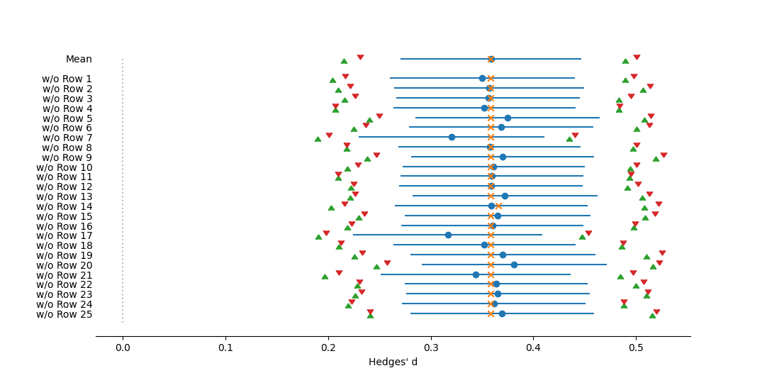
Forest plot of mean effect sizes from a jackknife meta-analysis, with the summary repeated with each study removed, one by one. Effect size measured as Hedges' d. The dotted vertical line represents no effect, or a mean of zero. Circles represent mean effect size, with the corresponding line the 95% confidence interval. X's represent the median. Upward-pointing triangles mark the confidence interval from a bootstrap (999 iterations) procedure, following Adams et al. (1997); downward-pointing triangles mark the bias-corrected bootstrap interval.References
Adams, D.C., J. Gurevitch, and M.S. Rosenberg (1997) Resampling tests for meta-analysis of ecological data. Ecology 78:1277–1283.
Cumulative Meta-Analysis
Cumulative Meta-Analysis (Chalmers 1991) is a process by which one performs an analysis on just two studies, then repeats by adding one additional study until all studies have been included. It's generally used to show when an effect has become stabilized.
Running a Cumulative Meta-Analysis
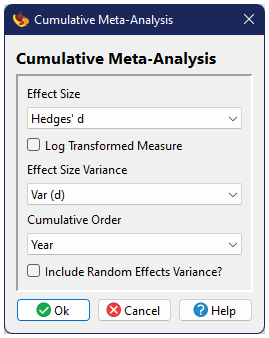
The options for a Cumulative Meta-Analysis are essentially identical to the Basic Analysis, except that the Failsafe Number tests are not included and a data column must be specified which contains the order in which the studies should be added. Traditionally this variable would represent time, but other options are possible.
Output
The output for a Cumulative Meta-Analysis is similar to that from a Basic Analysis, except that the tables of heterogenities and means are shown for each step in the cumulative analysis. The other primary difference is in the graphical output, if requested. In a Basic Analysis, the forest plot illustrates the global mean as well as the individual effect size for each study. In the Cumulative analysis the plot illustrates the change in estimated mean as more and more studies are added (from top to bottom), with the final mean equal to the global mean including all studies.
Analysis
Cumulative Meta-Analysis
→ Citation: Chalmers (1991)→ Effect Sizes: Hedges' d
→ Effect Size Variances: Var (d)
→ Cumulative Order: Year
→ Fixed Effects Model→ Standard confidence intervals around means based on Normal distribution
→ Use bootstrap for confidence intervals around means: 999 iterations
→ Citations: Adams et al. (1997), Dixon (1993)25 studies will be included in this analysis
Cumulative Results
Heterogeneity
     Source            Q      df   P(χ2)
-----------------------------------------
2 studies Qtotal     0.0088    1   0.9253
3 studies Qtotal     0.1264    2   0.9387
4 studies Qtotal     0.2893    3   0.9620
5 studies Qtotal     0.6159    4   0.9613
6 studies Qtotal     0.7839    5   0.9780
7 studies Qtotal     0.9891    6   0.9860
8 studies Qtotal     1.0607    7   0.9938
9 studies Qtotal     1.3277    8   0.9952
10 studies Qtotal    1.6082    9   0.9963
11 studies Qtotal    2.4313   10   0.9918
12 studies Qtotal    2.6697   11   0.9944
13 studies Qtotal    3.1745   12   0.9942
14 studies Qtotal    3.5687   13   0.9950
15 studies Qtotal    7.0163   14   0.9341
16 studies Qtotal    7.6698   15   0.9363
17 studies Qtotal    9.6369   16   0.8849
18 studies Qtotal   10.1785   17   0.8960
19 studies Qtotal   11.0756   18   0.8911
20 studies Qtotal   14.8515   19   0.7320
21 studies Qtotal   16.7843   20   0.6669
22 studies Qtotal   28.5583   21   0.1250
23 studies Qtotal   30.9686   22   0.0968
24 studies Qtotal   43.9570   23   0.0053
25 studies Qtotal   46.5517   24   0.0038
Mean Effect Sizes
                       n     Mean     Median         95% CI            Bootstrap CI      Bias-corrected CI
-----------------------------------------------------------------------------------------------------------
2 studies Hedges' d     2   -0.1402   -0.1524   -0.4871 to 0.2067   -0.1524 to -0.1176   -0.1524 to -0.1402
3 studies Hedges' d     3   -0.1030   -0.1176   -0.3773 to 0.1712   -0.1524 to -0.0411   -0.1524 to -0.0584
4 studies Hedges' d     4   -0.0761   -0.0411   -0.3173 to 0.1650   -0.1402 to -0.0110   -0.1471 to -0.0163
5 studies Hedges' d     5   -0.0412   -0.0411   -0.2506 to 0.1681    -0.1106 to 0.0271    -0.1173 to 0.0271
6 studies Hedges' d     6   -0.0277   -0.0411   -0.2267 to 0.1713    -0.1001 to 0.0519    -0.1030 to 0.0431
7 studies Hedges' d     7   -0.0120    0.0155   -0.1990 to 0.1751    -0.0884 to 0.0574    -0.0892 to 0.0570
8 studies Hedges' d     8   -0.0066    0.0155   -0.1896 to 0.1763    -0.0740 to 0.0690    -0.0765 to 0.0674
9 studies Hedges' d     9    0.0126    0.0655   -0.1550 to 0.1803    -0.0575 to 0.0767    -0.0613 to 0.0734
10 studies Hedges' d   10    0.0291    0.0655   -0.1270 to 0.1853    -0.0389 to 0.0916    -0.0418 to 0.0885
11 studies Hedges' d   11    0.0549    0.1000   -0.0910 to 0.2008    -0.0212 to 0.1239    -0.0208 to 0.1251
12 studies Hedges' d   12    0.0617    0.1000   -0.0817 to 0.2050    -0.0120 to 0.1344    -0.0108 to 0.1358
13 studies Hedges' d   13    0.0751    0.1070   -0.0634 to 0.2136    -0.0005 to 0.1435    -0.0012 to 0.1422
14 studies Hedges' d   14    0.0837    0.1070   -0.0522 to 0.2196     0.0119 to 0.1557     0.0005 to 0.1490
15 studies Hedges' d   15    0.1440    0.1140    0.0239 to 0.2640     0.0251 to 0.2403     0.0324 to 0.2474
16 studies Hedges' d   16    0.1550    0.1371    0.0380 to 0.2721     0.0441 to 0.2487     0.0515 to 0.2560
17 studies Hedges' d   17    0.1867    0.2317    0.0784 to 0.2951     0.0766 to 0.2674     0.0842 to 0.2725
18 studies Hedges' d   18    0.1929    0.2317    0.0858 to 0.2999     0.0763 to 0.2779     0.0805 to 0.2842
19 studies Hedges' d   19    0.2026    0.2317    0.0974 to 0.3077     0.0966 to 0.2812     0.1082 to 0.2845
20 studies Hedges' d   20    0.2382    0.2631    0.1394 to 0.3371     0.1215 to 0.3309     0.1265 to 0.3346
21 studies Hedges' d   21    0.2546    0.3043    0.1585 to 0.3507     0.1419 to 0.3365     0.1419 to 0.3372
22 studies Hedges' d   22    0.3057    0.3585    0.2141 to 0.3972     0.1788 to 0.4223     0.1875 to 0.4348
23 studies Hedges' d   23    0.3131    0.3585    0.2220 to 0.4042     0.1824 to 0.4279     0.2024 to 0.4406
24 studies Hedges' d   24    0.3523    0.3585    0.2638 to 0.4409     0.2142 to 0.4916     0.2299 to 0.5072
25 studies Hedges' d   25    0.3588    0.3585    0.2706 to 0.4470     0.2352 to 0.4925     0.2406 to 0.5015
References
Adams, D.C., J. Gurevitch, and M.S. Rosenberg (1997) Resampling tests for meta-analysis of ecological data. Ecology 78:1277–1283.
Chalmers, T.C. (1991) Problems induced by meta-analyses. Statistics in Medicine 10:971–980.
Dixon, P.M. (1993) The bootstrap and the jackknife: Describing the precision of ecological indices. Pp. 290—318 in Design and Analysis of Ecological Experiments, S.M. Scheiner and J. Gurevitch, eds. Chapman and Hall, New York.
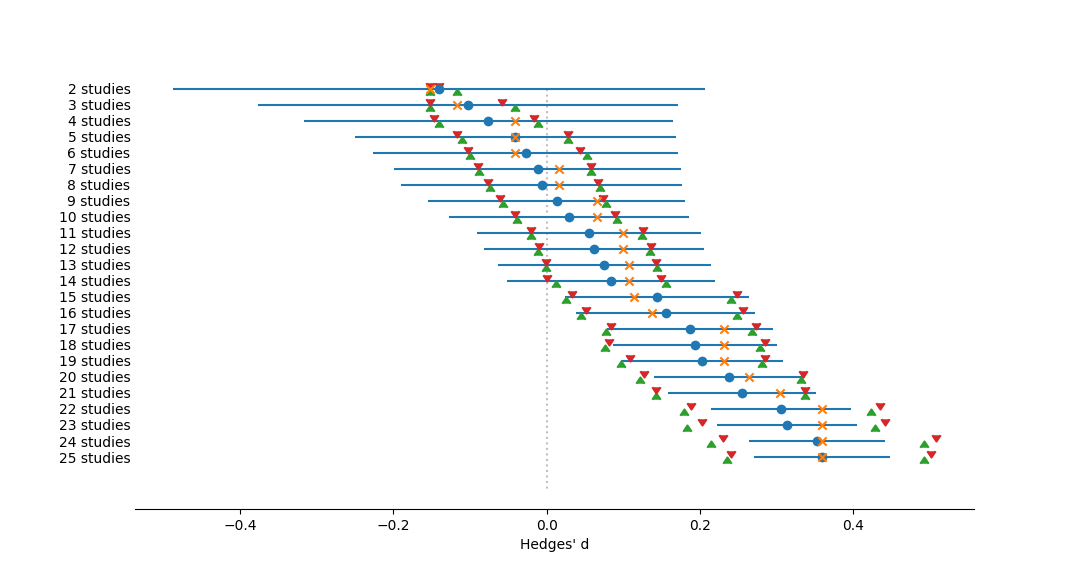
Forest plot of effect sizes from a cumulative meta-analysis, ranging from the fewest studies at the top to the most at the bottom, ordered by Year. Effect size measured as Hedges' d. The dotted vertical line represents no effect, or a mean of zero. Circles represent mean effect size, with the corresponding line the 95% confidence interval. X's represent the median. Upward-pointing triangles mark the confidence interval from a bootstrap (999 iterations) procedure, following Adams et al. (1997); downward-pointing triangles mark the bias-corrected bootstrap interval.
References
Adams, D.C., J. Gurevitch, and M.S. Rosenberg (1997) Resampling tests for meta-analysis of ecological data. Ecology 78:1277–1283.
Grouped Meta-Analysis
Grouped meta-analysis goes beyond the single global mean of the basic analysis and examines the mean effect size when studies are divided into two or more groups or categories. This type of analysis is conceptually similar to ANVOA. Structurally, the \(n\) studies are divided into \(k\) groups, where the jth group contains \(n_j\) studies.
Global means and variances are calculated just as in a basic analysis, but additionally, each group has its own mean, variance, and confidence interval calculated, using the same equations as in the basic analysis, except that studies are restricted to the group. The Q statistic for each indiviudal group is generally considered to be within-group heterogeneity, while the sum of these Q's is the total within-group heterogeneity, QW (or more generally referred to as the model heterogeneity, QM).
The difference between the total heterogeneity (QT) and the within (model) heterogeneity (QW or QM) is the between-group heterogeneity, QB (or more generally referred to as the error heterogeneity, QE).
$$Q_T = Q_M + Q_E, \text{ or alternatively, } Q_W + Q_B.$$
Note that QB/QE can also be calculated as the weighted sum of squares differences between the group means and the global mean, where each group mean is weighted by the sum of the weights of the studies within the group, or
$$Q_B = \sum{\sum{w_{ij}\left(\bar{\theta}_j - \bar{\theta}\right)^2}},$$
where \(\bar{\theta}_j\) is the mean of the jth group and \(w_{ij}\) is the weight of the ith study in the jth group.
The total, model (within), and error (between) group heterogeneities can be compared in an ANOVA like table, where each value is compared to a χ2 distribution with \(k-1\), \(n-k\), and \(n-1\) degrees of freedom.
| Source of Heterogeneity | Symbol | df | Equation |
|---|---|---|---|
| Model | \(Q_M\) | \(k-1\) | \(\sum{\sum{w_{ij}\left(\theta_{ij} - \bar{\theta}_j\right)^2}}\) |
| Error | \(Q_E\) | \(n-k\) | \(\sum{\sum{w_{ij}\left(\bar{\theta}_j - \bar{\theta}\right)^2}}\) |
| Total | \(Q_T\) | \(n-1\) | \(\sum{\sum{w_{ij}\left(\theta_{ij} - \bar{\theta}\right)^2}}\) |
Alternatively, the significance of the model (the group structure) can be tested through a randomization test where the association between specific studies and the group they belong to is randomized.
For a random effects model, the estimate of pooled variance is dependent on the model structure; for this type of analysis (often referred to as a mixed-effects model) the estimate is determined by
$$\hat{\sigma}^2 = \frac{Q_E - (n - k)}{\sum\limits_{j=1}^k{\left[ \sum\limits_{i=1}^{n_k}w_{ij} - \frac{\sum\limits_{i=1}^{n_k}{{w_{ij}^2}}}{\sum\limits_{i=1}^{n_k}w_{ij}}\right]}}.$$
As before, when conducting a random-effects model, the weights are recalculated as
$$w_i^* = 1/{\left(v_i + \hat{\sigma}^2\right)} ,$$
and the rest of the calculations repeated using these new weights.
Running a grouped analysis
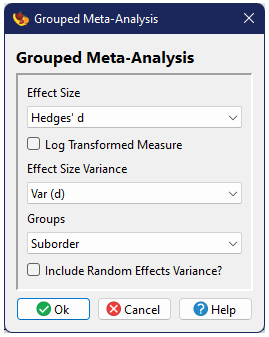
The options for a Grouped Meta-Analysis are similar to the Basic Analysis, except that the Failsafe Number tests are not included and a data column must be specified which contains the group structure. This column can contain numbers or text; studies with the same value would be considered to be in the same group.
Data Requirement: Each group included in the analysis must contain at least two studies. If a group appears to contain only one study, the analysis will not be conducted and the output will identify the groups with too few studies. Studies in these groups can be filtered in order to run the analysis on those groups which do have at least two studies present.
The one other difference is the addition of an option to test the significance of the model through a randomization test. This test is conducted independently of bootstrapping, if chosen.
Output
The output for a Grouped Meta-Analysis includes group specific output, as well as the same general output found in a Basic Analysis. The graphical output, if requested, is a forest plot which shows the global mean and the group means.
Analysis
Structure: Grouped
→ Citation: Hedges and Olkin (1985)→ Effect Sizes: Hedges' d
→ Effect Size Variances: Var (d)
→ Groups: Suborder
→ Fixed Effects Model→ Standard confidence intervals around means based on Normal distribution
→ Use bootstrap for confidence intervals around means: 999 iterations
→ Citations: Adams et al. (1997), Dixon (1993)→ Use randomization to test model structure: 999 iterations
→ Citation: Adams et al. (1997)25 studies will be included in this analysis
Group Results
Heterogeneity
       Source             Q      df   P(χ2)
--------------------------------------------
Heterocera (within)    40.3206   17   0.0012
Rhopalocera (within)    6.1872    6   0.4026
Source I2 95% CI --------------------------------------------------- Heterocera (within) 57.8379 28.8567 to 75.0132 Rhopalocera (within) 3.0254 0.0000 to 28.1177→ Citations: Higgins and Thompson (2002), Huedo-Medina et al. (2006)
    Source           Q      df   P(χ2)    P(randomization)
----------------------------------------------------------
Model (Between)    0.0439    1   0.8340             0.2470
Error (Within)    46.5078   23   0.0026
---------------------------------------------------------------------
Total             46.5517   24   0.0038
Mean Effect Sizes
                        n     Mean    Median        95% CI          Bootstrap CI     Bias-corrected CI
------------------------------------------------------------------------------------------------------
Heterocera Hedges' d    18   0.3627   0.3585   0.2675 to 0.4579   0.2004 to 0.5169    0.2148 to 0.5335
Rhopalocera Hedges' d    7   0.3356   0.2317   0.1014 to 0.5698   0.2006 to 0.6005    0.2045 to 0.6207
Global Results
Heterogeneity
Source      Q      df   P(χ2)
------------------------------
Total    46.5517   24   0.0038
→ Citation: Hedges and Olkin (1985)
Source     I2            95% CI
-------------------------------------
Total    48.4444   17.9350 to 67.6113
→ Citations: Higgins and Thompson (2002), Huedo-Medina et al. (2006)
Mean Effect Size
                   n     Mean    Median        95% CI          Bootstrap CI     Bias-corrected CI
-------------------------------------------------------------------------------------------------
Global Hedges' d   25   0.3588   0.3585   0.2706 to 0.4470   0.2144 to 0.4868    0.2305 to 0.4992
Sqrt Pooled Variance = 0.2293
Mean Study Variance = 0.0838
ratio = 2.7361References
Adams, D.C., J. Gurevitch, and M.S. Rosenberg (1997) Resampling tests for meta-analysis of ecological data. Ecology 78:1277–1283.
Dixon, P.M. (1993) The bootstrap and the jackknife: Describing the precision of ecological indices. Pp. 290—318 in Design and Analysis of Ecological Experiments, S.M. Scheiner and J. Gurevitch, eds. Chapman and Hall, New York.
Hedges, L.V. and I. Olkin (1985) Statistical Methods for Meta-analysis. Academic Press, Orlando, FL.
Higgins, J.P.T. and S.G. Thompson (2002) Quantifying heterogeneity in a meta-analysis. Statistics in Medicine 21:1539–1558.
Huedo-Medina, T.B., J. Sánchez-Meca, F. Marín-Martínez, and J. Botella (2006) Assessing heterogeneity in meta-analysis: Q statistic or I2 index? Psychological Methods 11:193–206.
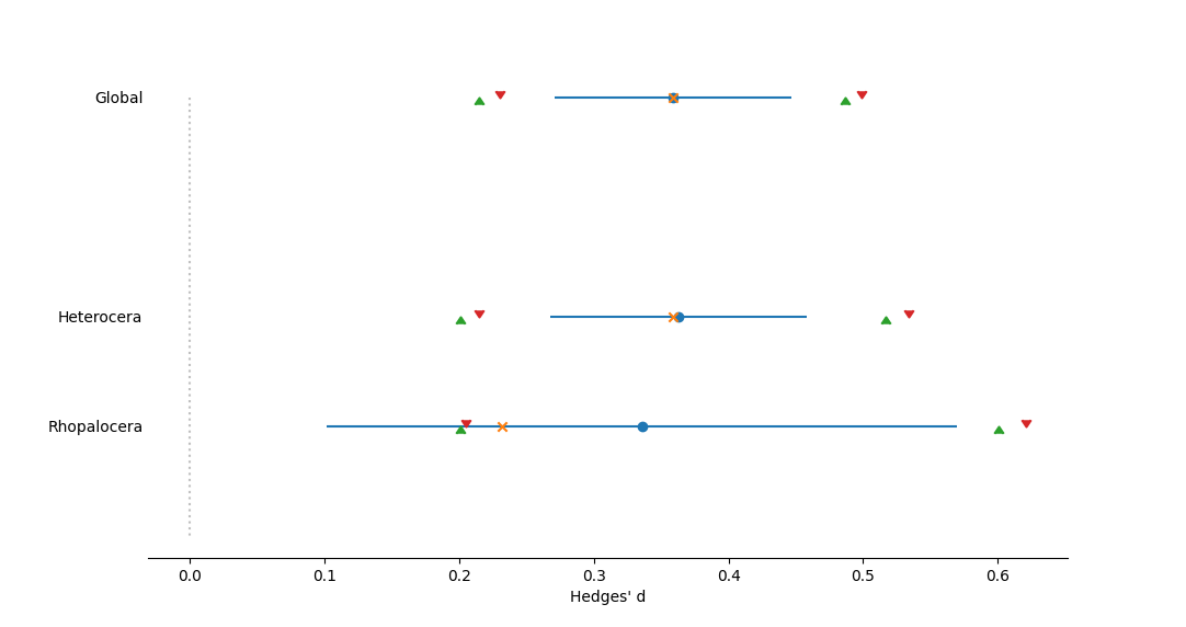
Forest plot of effect sizes for the mean of all studies, as well as subgroups of studies designated by Suborder. Effect size measured as Hedges' d. The dotted vertical line represents no effect, or a mean of zero. Circles represent mean effect size, with the corresponding line the 95% confidence interval. X's represent the median. Upward-pointing triangles mark the confidence interval from a bootstrap (999 iterations) procedure, following Adams et al. (1997); downward-pointing triangles mark the bias-corrected bootstrap interval.
References
Adams, D.C., J. Gurevitch, and M.S. Rosenberg (1997) Resampling tests for meta-analysis of ecological data. Ecology 78:1277–1283.
Nested Group Meta-Analysis
Nested group meta-analysis is similar to nested ANOVA in the same manner that Grouped Meta-Analysis is similar to one-way ANVOA. In nested meta-analysis there are two or more levels of groupings, but the groupings are specifically nested within one another rather than independent (as one would find a two or more way ANOVA).
Mathematically, the procedure for Nested group meta-analysis is very similar to that of Grouped Meta-Analysis, in that one can calculate means, variances, and within-group heterogeneities for each group at each level, and then compare different levels of nesting by contrasting means at one level with means at a higher level (Rosenberg 2013).
The major catch with a nested analysis is that a random-effects model is not possible, at least with the least-squares/moments approach for calculations used in . For this particular analysis option, only fixed-effects models are implemented.
Running a Nested Group Meta-Analysis
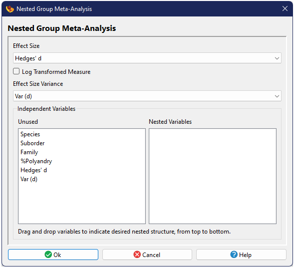
The dialog for a Nested Grouped Meta-Analysis is a bit different from those already described. While the basic options are the same (except for the absence of the random effects model), the bottom of the first dialog window contains two boxes, starting with the one on the left listing all columns and the one on the right blank. The right box will contain the nesting structure, with the top level group first, followed by second, third, etc. To create this structure, you can drag and drop names between the two boxes.
Data Requirement: Each group included in the analysis, at every level, must contain at least two studies. If a group appears to contain only one study, the analysis will not be conducted and the output will identify the group with too few studies. Studies in these groups can be filtered in order to run the analysis on those groups which do have at least two studies present. may not be able to detect all problematic groups at a time, so multiple attempts to run/filter may be necessary to meet the data requirement.
The secondary options for nested group meta-analysis are identical to those of Grouped Meta-Analysis, with bootstrapping and randomization tests, and graphical output.
Output
The output for a Nested Grouped Meta-Analysis includes group specific output, as well as the same general output found in a Basic Analysis. The graphical output, if requested, is a forest plot which shows the global mean and the group means. Data tables and the figure represent nesting by the presence of an arrow (→). Multiple arrows indicate multiple levels of nesting.
Analysis
Structure: Nested Groups
→ Citation: Rosenberg (2013)→ Effect Sizes: Hedges' d
→ Effect Size Variances: Var (d)
→ Nested Variables (top to bottom): Suborder, Family
→ Fixed Effects Model→ Use bootstrap for confidence intervals around means: 999 iterations
→ Citations: Adams et al. (1997), Dixon (1993)→ Standard confidence intervals around means based on Normal distribution
→ Use randomization to test model structure: 999 iterations
→ Citation: Adams et al. (1997)Pre-filtered studies excluded from analysis: Row 1, Row 12, Row 23
22 studies will be included in this analysis
Group Results
Heterogeneity
         Source                Q      df   P(χ2)
-------------------------------------------------
Heterocera (within)         39.5798   16   0.0009
  → Gelechiidae (within)     2.0062    1   0.1567
  → Noctuidae (within)       4.9239    5   0.4252
  → Pyralidae (within)       3.0375    3   0.3859
  → Tortricidae (within)    19.1049    4   0.0007
Rhopalocera (within)         5.3599    4   0.2523
  → Papilionidae (within)    0.0018    1   0.9662
  → Pieridae (within)        3.0609    2   0.2164
Source Q df P(χ2) P(randomization) -------------------------------------------------------- Qm (Suborder) 0.0653 1 0.7983 0.9820 Qm (Family) 12.8045 4 0.0123 0.4960 Qe 32.1352 16 0.0096 ------------------------------------------------------------------- Total 45.0050 21 0.0017Mean Effect Sizes
                             n     Mean    Median        95% CI           Bootstrap CI      Bias-corrected CI
-------------------------------------------------------------------------------------------------------------
Heterocera Hedges' d         17   0.3527   0.3585    0.2549 to 0.4506    0.1818 to 0.5182    0.1905 to 0.5248
  → Gelechiidae Hedges' d     2   0.6515   0.5072    0.4428 to 0.8601    0.5072 to 0.8090    0.5072 to 0.6515
  → Noctuidae Hedges' d       6   0.2450   0.3762    0.0584 to 0.4316    0.0070 to 0.3776    0.0070 to 0.3788
  → Pyralidae Hedges' d       4   0.2441   0.3585    0.0546 to 0.4335    0.0415 to 0.3698    0.0168 to 0.3698
  → Tortricidae Hedges' d     5   0.3228   0.0655    0.1222 to 0.5233   -0.0145 to 0.7536   -0.0122 to 0.7661
Rhopalocera Hedges' d         5   0.3936   0.2317    0.0955 to 0.6917    0.2106 to 0.8675    0.2106 to 0.8675
  → Papilionidae Hedges' d    2   0.2358   0.2317   -0.1254 to 0.5971    0.2317 to 0.2506    0.2317 to 0.2506
  → Pieridae Hedges' d        3   0.7304   1.0125    0.2026 to 1.2582    0.1105 to 1.1690    0.1105 to 1.1090
Global Results
Heterogeneity
Source      Q      df   P(χ2)
------------------------------
Total    45.0050   21   0.0017
→ Citation: Hedges and Olkin (1985)
Source     I2            95% CI
-------------------------------------
Total    53.3385   24.2595 to 71.2532
→ Citations: Higgins and Thompson (2002), Huedo-Medina et al. (2006)
Mean Effect Size
                   n     Mean    Median        95% CI          Bootstrap CI     Bias-corrected CI
-------------------------------------------------------------------------------------------------
Global Hedges' d   22   0.3567   0.3585   0.2580 to 0.4553   0.2096 to 0.4883    0.2226 to 0.5024
Sqrt Pooled Variance = 0.0000
Mean Study Variance = 0.0864
ratio = 0.0000References
Adams, D.C., J. Gurevitch, and M.S. Rosenberg (1997) Resampling tests for meta-analysis of ecological data. Ecology 78:1277–1283.
Dixon, P.M. (1993) The bootstrap and the jackknife: Describing the precision of ecological indices. Pp. 290—318 in Design and Analysis of Ecological Experiments, S.M. Scheiner and J. Gurevitch, eds. Chapman and Hall, New York.
Hedges, L.V. and I. Olkin (1985) Statistical Methods for Meta-analysis. Academic Press, Orlando, FL.
Higgins, J.P.T. and S.G. Thompson (2002) Quantifying heterogeneity in a meta-analysis. Statistics in Medicine 21:1539–1558.
Huedo-Medina, T.B., J. Sánchez-Meca, F. Marín-Martínez, and J. Botella (2006) Assessing heterogeneity in meta-analysis: Q statistic or I2 index? Psychological Methods 11:193–206.
Rosenberg, M.S. (2013) Moment and least-squares based approaches to meta-analytic inference. Pp. 108–124 in Handbook of Meta-analysis in Ecology and Evolution, J. Koricheva, J. Gurevitch and K.L. Mengersen, eds. Princeton University Press: Princeton, NJ.
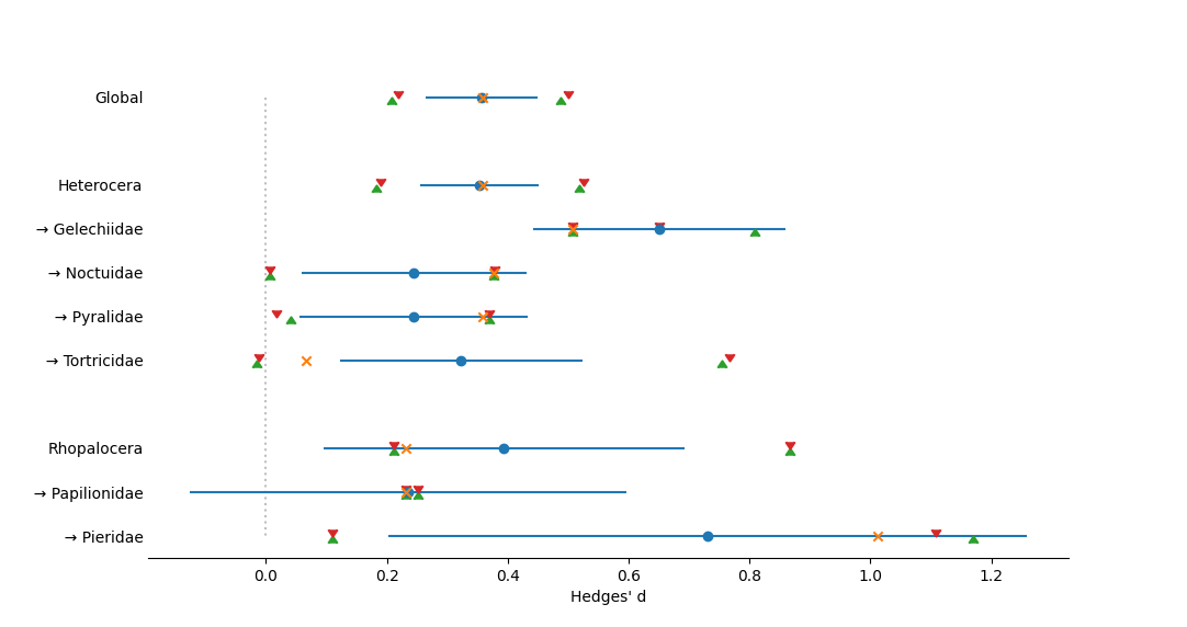
Forest plot of effect sizes for the mean of all studies as well as nested subgroups. Arrows in front of labels along the y-axis indicate the degree of nesting. Effect size measured as Hedges' d. The dotted vertical line represents no effect, or a mean of zero. Circles represent mean effect size, with the corresponding line the 95% confidence interval. X's represent the median. Upward-pointing triangles mark the confidence interval from a bootstrap (999 iterations) procedure, following Adams et al. (1997); downward-pointing triangles mark the bias-corrected bootstrap interval.
References
Adams, D.C., J. Gurevitch, and M.S. Rosenberg (1997) Resampling tests for meta-analysis of ecological data. Ecology 78:1277–1283.
Linear Meta-Regression Analysis
Linear Meta-Regression Analysis examines the relationship between the effecct size and an independent variable in a typical regression framework, estimating the parameters for the equation
$$\theta_i = \beta_0 + \beta_1 x_i + \epsilon_i,$$
where \(\beta_0\) is the intercept, \(\beta_1\) is the slope, and \(x_i\) is the independent variable. The equations for estimating the slope and intercept are:
$$\beta_1 = \frac{\sum{w_i x_i \theta_i} - \frac{\sum{w_i x_i} \sum{w_i \theta_i}}{\sum{w_i}}}{\sum{w_i x_i^2} - \frac{\left(\sum{w_i x_i} \right)^2}{\sum{w_i}}}$$
and
$$\beta_0 = \frac{\sum{w_i \theta_i} - \beta_1 \sum{w_i x_i}}{\sum{w_i}},$$
with standard errors of
$$s_{\beta_1} = \frac{1}{\sum{w_i x_i^2} - \frac{\left(\sum{w_i x_i} \right)^2}{\sum{w_i}}}$$
and
$$s_{\beta_0} = \frac{1}{\sum{w_i} - \frac{\left(\sum{w_i x_i}\right)^2}{\sum{w_i x_i^2}}},$$
respectively (Hedges and Olkin 1985; Greenland 1987). The heterogeneity of the regression model, QM, which has one degree of freedom, can be estimated as the square of the slope over the square of its standard error, or
$$Q_M = \frac{\beta_1^2}{s_{\beta_1}^2}.$$
Total heterogeneity can be estimated as normal and the error heterogeneity is once again the difference between the total and the model, allowing us to create a heterogeneity table for regression much like that of other analyses:
| Source of Heterogeneity | Symbol | df | Equation |
|---|---|---|---|
| Model | \(Q_M\) | 1 | \(\frac{\beta_1^2}{s_{\beta_1}^2}\) |
| Error | \(Q_E\) | \(n-2\) | \(Q_T - Q_M\) |
| Total | \(Q_T\) | \(n-1\) | \(\sum{w_{i}\left(\theta_{i} - \bar{\theta}\right)^2}\) |
Alternatively, the significance of the model (the group structure) can be tested through a randomization test where the association between specific studies and the independent variable is randomized.
For a random effects model, the estimate of pooled variance is dependent on the model structure; for this type of analysis the estimate is determined by (Rosenberg et al. 2000; Rosenberg 2013):
$$\hat{\sigma}^2 = \frac{Q_E - \left(n - 2\right)}{\sum\limits_{i=1}^n{w_i} - \sum\limits_{j=1}^n{w_j^2}\left[\frac{\sum\limits_{i=1}^n{w_i x_i^2} - 2x_j\sum\limits_{i=1}^n{w_i x_i} + x_j^2\sum\limits_{i=1}^n{w_i}}{\sum\limits_{i=1}^n{w_i} \sum\limits_{i=1}^n{w_i x_i^2} - \left(\sum\limits_{i=1}^n{w_i x_i} \right)^2} \right]}.$$
As before, when conducting a random-effects model, the weights are recalculated as
$$w_i^* = 1/{\left(v_i + \hat{\sigma}^2\right)} ,$$
and the rest of the calculations repeated using these new weights.
Running a regression analysis
The options for a Linear Regression Meta-Analysis are similar to the Basic Analysis, except that a data column must be specified which contains the independent variable.
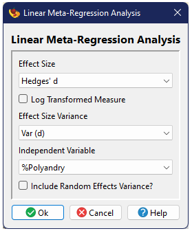
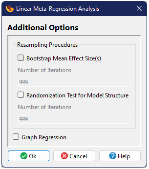
The one other difference is the addition of an option to test the significance of the model through a randomization test. This test is conducted independently of bootstrapping, if chosen.
Output
The output for a Linear Regression Meta-Analysis includes information on the predictors (intercept and slope), a heterogeneity model table, as well as the same general output found in a Basic Analysis. The graphical output, if requested, is a scatter plot of the effect sizes vs. independent variables, including the regression line.
Analysis
Structure: Linear Regression
→ Citations: Hedges and Olkin (1985), Greenland (1987)→ Effect Sizes: Hedges' d
→ Effect Size Variances: Var (d)
→ Independent Variable: %Polyandry
→ Fixed Effects Model→ Standard confidence intervals around means based on Normal distribution
→ Use bootstrap for confidence intervals around means: 999 iterations
→ Citations: Adams et al. (1997), Dixon (1993)→ Use randomization to test model structure: 999 iterations
→ Citation: Adams et al. (1997)Studies with invalid data: Row 3, Row 10, Row 16
22 studies will be included in this analysis
Regression Results
Predictors
Predictor   Value      SE     P(Normal)
---------------------------------------
Intercept   0.1161   0.0918      0.2059
Slope       0.0059   0.0019      0.0021
Heterogeneity
Source      Q      df   P(χ2)    P(randomization)
-------------------------------------------------
Model     9.4576    1   0.0021             0.3230
Error    36.5623   20   0.0132
------------------------------------------------------------
Total    46.0199   21   0.0013
Global Results
Heterogeneity
Source      Q      df   P(χ2)
------------------------------
Total    46.0199   21   0.0013
→ Citation: Hedges and Olkin (1985)
Source     I2            95% CI
-------------------------------------
Total    54.3676   26.1112 to 71.8182
→ Citations: Higgins and Thompson (2002), Huedo-Medina et al. (2006)
Mean Effect Size
                   n     Mean    Median        95% CI          Bootstrap CI     Bias-corrected CI
-------------------------------------------------------------------------------------------------
Global Hedges' d   22   0.3601   0.3585   0.2697 to 0.4505   0.2117 to 0.5022    0.2122 to 0.5050
Sqrt Pooled Variance = 0.2008
Mean Study Variance = 0.0754
ratio = 2.6649References
Adams, D.C., J. Gurevitch, and M.S. Rosenberg (1997) Resampling tests for meta-analysis of ecological data. Ecology 78:1277–1283.
Dixon, P.M. (1993) The bootstrap and the jackknife: Describing the precision of ecological indices. Pp. 290—318 in Design and Analysis of Ecological Experiments, S.M. Scheiner and J. Gurevitch, eds. Chapman and Hall, New York.
Greenland, S. (1987) Quantitative methods in the review of epidemiologic literature. Epidemiologic Review 9:1–30.
Hedges, L.V. and I. Olkin (1985) Statistical Methods for Meta-analysis. Academic Press, Orlando, FL.
Higgins, J.P.T. and S.G. Thompson (2002) Quantifying heterogeneity in a meta-analysis. Statistics in Medicine 21:1539–1558.
Huedo-Medina, T.B., J. Sánchez-Meca, F. Marín-Martínez, and J. Botella (2006) Assessing heterogeneity in meta-analysis: Q statistic or I2 index? Psychological Methods 11:193–206.
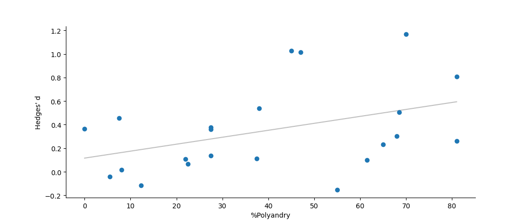
Plot of Hedges' d vs. %Polyandry, with a fixed effects meta-analytic linear regression following the methods of Hedges and Olkin (1985) and Greenland (1987).
References
Greenland, S. (1987) Quantitative methods in the review of epidemiologic literature. Epidemiologic Review 9:1–30.
Hedges, L.V. and I. Olkin (1985) Statistical Methods for Meta-analysis. Academic Press, Orlando, FL.
Complex/GLM Meta-Analysis
Previous analyses mostly allowed examination of effect sizes with simple structural models, either one-way grouping or univariate regression. The Complex/GLM framework allows any number of explanatory variables, including two-or-more independent groupings (as in a two-or-more way ANOVA), multivariate regression, or a combination of both in an ANCOVA or MANCOVA-like framework. This analysis is conducted in a generalized regression framework, where we are estimating parameters for the equation
$$\theta_i = \beta_0 + \beta_1 x_{1i} + \beta_2 x_{2i} + \beta_3 x_{3i}...,$$
with the number of predictors dependent on the desired model structure. The first predictor is a constant (intercept), while each continuous variable contributes one predictor, and each grouping variable contributes \(k-1\) predictors, where \(k\) is the number of groups for that particular variable. If this analysis is run without any parameters but the constant, it is equivalent to a basic meta-analysis and \(\beta_0\) is the global mean. If it is run with a single continuous variable, it is equivalent to a linear meta-regression and \(\beta_0\) and \(\beta_1\) are the intercept and slope. If it is run with a single group column, it is equivalent to a grouped meta-analysis, although interpretation of the predictors is slightly more complicated as they represent contrasts among groups.
This meta-analytic framework is computed using matrix algebra. The effect sizes are placed in a column vector \(\boldsymbol{\theta}\), while the continuous and categorical variables are placed in a matrix called \(\boldsymbol{X}\) which includes a column of 1's (for the constant), a column for each continuous variable, and \(k-1\) columns for each group in each categorical variable. In matrix notation form we are estimating parameters for the equation
$$\boldsymbol{\theta} = \boldsymbol{\beta X} + \boldsymbol{E},$$
where \(\boldsymbol{\beta}\) contains the predictor (regression) coefficients. To solve this we use a weighted-GLM approach, where the matrix \(\boldsymbol{W}\) is an n×n matrix with the individual study weights on the diagonal and the rest of the matrix containing zeros. From this we can calculate \(\boldsymbol{\beta}\) as
$$\boldsymbol{\beta} = \left( \boldsymbol{X}^T \boldsymbol{W} \boldsymbol{X}\right)^{-1} \boldsymbol{X}^T \boldsymbol{W} \boldsymbol{\theta}.$$
The variance of each component of \(\boldsymbol{\beta}\) can be calculated as
$$\boldsymbol{\Sigma_{\beta}} = \left( \boldsymbol{X}^T \boldsymbol{W} \boldsymbol{X}\right)^{-1},$$
where the variance is the corresponding element of the diagonal of \(\boldsymbol{\Sigma_{\beta}}\). If \(\boldsymbol{\beta^*}\) is simply \(\boldsymbol{\beta}\) with the first value removed, and \(\boldsymbol{\Sigma_{\beta}^*}\) is \(\boldsymbol{\Sigma_{\beta}}\) with the first row and column removed, then the model heterogeneity can be determined as:
$$Q_M = \boldsymbol{\beta^{*T}} {\boldsymbol{\Sigma_{\beta}^{*}}}^{-1} \boldsymbol{\beta^*},$$
while the error heterogeneity can be calculated as
$$Q_E = \left(\boldsymbol{\theta} - \boldsymbol{X}\boldsymbol{\beta}\right)^T \boldsymbol{W} \left(\boldsymbol{\theta} - \boldsymbol{X}\boldsymbol{\beta}\right).$$
Total heterogeneity is most readily calculated as the sum of \(Q_M\) and \(Q_E\), and thus our model hetereogeneity table is
| Source of Heterogeneity | Symbol | df | Equation |
|---|---|---|---|
| Model | \(Q_M\) | p | \(\boldsymbol{\beta^{*T}} {\boldsymbol{\Sigma_{\beta}^{*}}}^{-1} \boldsymbol{\beta^*}\) |
| Error | \(Q_E\) | \(n-p-1\) | \(\left(\boldsymbol{\theta} - \boldsymbol{X}\boldsymbol{\beta}\right)^T \boldsymbol{W} \left(\boldsymbol{\theta} - \boldsymbol{X}\boldsymbol{\beta}\right)\) |
| Total | \(Q_T\) | \(n-1\) | \(Q_M + Q_E\) |
where p is the number of columns of \(\boldsymbol{X}\) minus one.
Alternatively, the significance of the model can be tested through a randomization test where the association between specific studies and the independent variables is randomized.
For a random effects model, the estimate of pooled variance is dependent on the model structure; for this type of analysis the estimate is determined by (Hedges and Olkin 1985; Rosenberg 2013):
$$\hat{\sigma}^2 = \frac{Q_E - \left(n - p - 1\right)}{\text{tr}\left(\boldsymbol{W}\right) - \text{tr}\left[\boldsymbol{W}\boldsymbol{X}\left(\boldsymbol{X}^T\boldsymbol{W}\boldsymbol{X}\right)^{-1}\boldsymbol{X}^T\boldsymbol{W}\right]},$$
where \(\text{tr}\left(\right)\) indicates the trace of the matrix. The other formulas for random effects variance presented earlier are simplifications of this general equation for specific conformations of \(\boldsymbol{X}\). As before, when conducting a random-effects model, the weights are recalculated as
$$w_i^* = 1/{\left(v_i + \hat{\sigma}^2\right)} ,$$
and the rest of the calculations repeated using these new weights.
Running a complex/GLM analysis
The options for a Complex/GLM Meta-Analysis are a bit more complex, as one can include any number of independent variables to the analysis. Beneath the standard options are three boxes, one indicating unused variables, one for categorical (grouping) variables, and one for continuous variables. The user can drag and drop variables among these categories to create the model structure they wish to conduct the meta-analysis under.
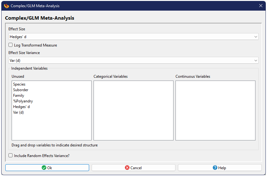
The additional options include bootstrapping confidence intervals around the mean, as well as a randomization test for model structure. Graphical output is not an option for the complex/glm analysis.
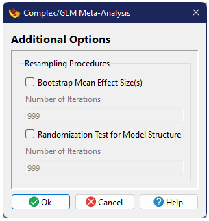
Output
The output for a Complex/GLM Meta-Analysis includes information on the predictors, a heterogeneity model table, as well as the same general output found in a Basic Analysis. No graphical output is produced as part of this analysis.
Analysis
Structure: Complex/GLM
→ Citations: Hedges and Olkin (1985), Rosenberg et al. (2000)→ Effect Sizes: Hedges' d
→ Effect Size Variances: Var (d)
→ Categorical Independent Variable(s): Suborder
→ Continuous Independent Variable(s): %Polyandry
→ Fixed Effects Model→ Standard confidence intervals around means based on Normal distribution
→ Use bootstrap for confidence intervals around means: 999 iterations
→ Citations: Adams et al. (1997), Dixon (1993)→ Use randomization to test model structure: 999 iterations
→ Citation: Adams et al. (1997)Studies with invalid data: Row 3, Row 10, Row 16
22 studies will be included in this analysis
Model Results
Predictors
   Predictor      Value      SE          95% CI         P(Normal)
-----------------------------------------------------------------
β0 (intercept)    0.1236   0.1042   -0.0807 to 0.3278      0.2358
β1 (%Polyandry)   0.0059   0.0019    0.0021 to 0.0097      0.0021
β2 (Suborder)     0.0106   0.0699   -0.1263 to 0.1475      0.8794
Heterogeneity
Source      Q      df   P(χ2)    P(randomization)
-------------------------------------------------
Model     9.4807    2   0.0087             0.2390
Error    36.5392   19   0.0091
------------------------------------------------------------
Total    46.0199   21   0.0013
Global Results
Heterogeneity
Source      Q      df   P(χ2)
------------------------------
Total    46.0199   21   0.0013
→ Citation: Hedges and Olkin (1985)
Source     I2            95% CI
-------------------------------------
Total    54.3676   26.1112 to 71.8182
→ Citations: Higgins and Thompson (2002), Huedo-Medina et al. (2006)
Mean Effect Size
                   n     Mean    Median        95% CI          Bootstrap CI     Bias-corrected CI
-------------------------------------------------------------------------------------------------
Global Hedges' d   22   0.3601   0.3585   0.2697 to 0.4505   0.2192 to 0.5069    0.2271 to 0.5283
Sqrt Pooled Variance = 0.2114
Mean Study Variance = 0.0754
ratio = 2.8047References
Adams, D.C., J. Gurevitch, and M.S. Rosenberg (1997) Resampling tests for meta-analysis of ecological data. Ecology 78:1277–1283.
Dixon, P.M. (1993) The bootstrap and the jackknife: Describing the precision of ecological indices. Pp. 290—318 in Design and Analysis of Ecological Experiments, S.M. Scheiner and J. Gurevitch, eds. Chapman and Hall, New York.
Hedges, L.V. and I. Olkin (1985) Statistical Methods for Meta-analysis. Academic Press, Orlando, FL.
Higgins, J.P.T. and S.G. Thompson (2002) Quantifying heterogeneity in a meta-analysis. Statistics in Medicine 21:1539–1558.
Huedo-Medina, T.B., J. Sánchez-Meca, F. Marín-Martínez, and J. Botella (2006) Assessing heterogeneity in meta-analysis: Q statistic or I2 index? Psychological Methods 11:193–206.
Rosenberg, M.S., D.C. Adams, and J. Gurevitch (2000) MetaWin: Statistical Software for Meta-analysis. Sinauer Associates, Sunderland, MA.
Phylogenetic GLM Meta-Analysis
Phylogenetic GLM Meta-Analysis is an analysis-type unique to the biological sciences, as it conducts a meta-analysis while accounting for the non-independence of multi-taxonomic studies due to shared phylogenetic history of the taxa. This method uses the approach of Lajeunesse (2009) and Lajeunesse et al. (2013).
Warning: The phylogenetic glm meta-analysis is still experimental and has some kinks that have not definitively been worked out yet. The help section will be written out when we are more confident of the results.
Graphs and Figures
Graphs and figures are created by through two mechanisms: (1) as an optional components of many analyses, or (2) directly through a choice from the menu. Whenever a figure is created, it will appear in the Graph Tab, along with an automatically generated caption.
Remember that any studies that have been marked for filtering will automatically be excluded from figures.
Scatter Plot
A scatter plot is simply a point plot of two continuous variables. One can use this plotting function to create funnel plots, although a more advanced funnel plot figure can be found under publication bias analyses.
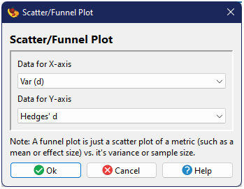
To draw a scatter plot, simply choose from the menu. From here you can choose the two variables to contrast and the figure will show up in the Graph Tab.
Output Example
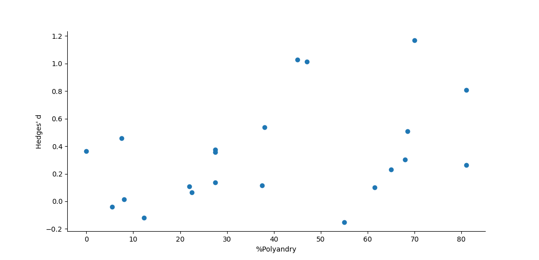
Scatter plot of Hedges' d vs. %Polyandry.
Weighted Histogram
A histogram is a bar plot illustrating the frequency of observations in a series of bins. A weighted histogram weights the count (frequency) of each observation. In meta-analysis you generally would create a histogram for effect sizes.
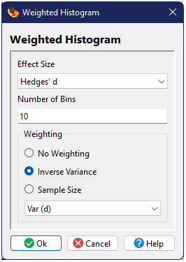
To draw a histogram, choose from the menu. From here you can specify the Effect Size and the number of bins to include, as well as whether you want the histogram to be unweighted, weighted by sample size, or weighted by the inverse of the variance (which is generally how weights are determined in meta-analysis). If either of the latter two options are chosen, the user can then specify the source of the sample size or weights. The figure will show up in the Graph Tab.
Output Example
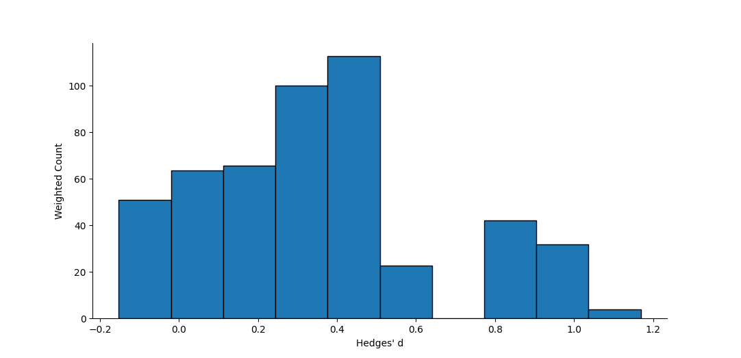
Histogram of Hedges' d from individual studies. Counts were weighted by the inverse of the variance of each effect size.
Forest Plot
A forest plot displays means and their confidence intervals for a series of observations or groups. A number of analyses in will optionally create forest plots, but this option allows the user to construct a forest plot for all of the input studies. Note that the figure can become overwhelmed with a large number of studies. To draw a forest plot, choose from the menu. From here you can specify the Effect Size and Variance.
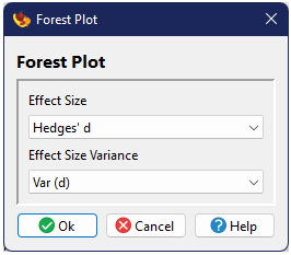
The figure will show up in the Graph Tab. The forest plot will stack each observation vertically, in the order they appear in the data matrix. The point indicates the observed effect size and the corresponding line it's 95% confidence interval based on the variance, with the corresponding study label (the row header) listed on the left side of the figure. A vertical silver dotted line marks an effect size of zero (generally the null hypothesis for standardized effect sizes).
The confidence interval can be modified by choosing a different significance level from the output options.
Output Example
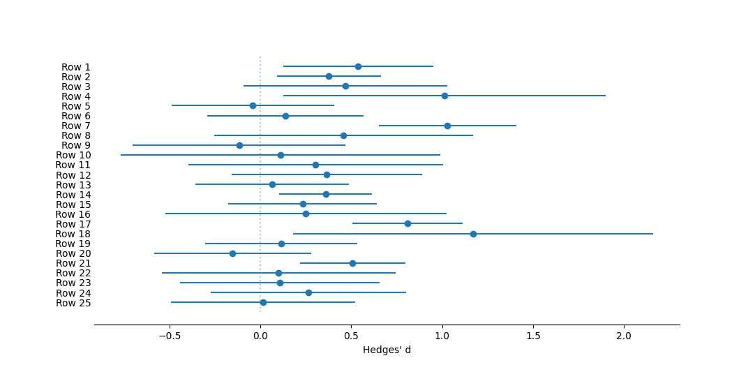
Forest plot of individual effect sizes for each study. Effect size measured as Hedges' d. The dotted vertical line represents no effect, or a mean of zero. Circles represent mean effect size, with the corresponding line the 95% confidence interval.
Normal Quantile Plot
The Normal Quantile Plot is as an alternative approach to looking for publication biases (Wang and Bushman, 1998). The normal quantile plot is a special case of a quantile quantile plot; this is a plot where two distributions are compared by plotting their quantiles against each other. If the two distributions are similar the quantiles will also be similar and the points will fall close to the line x = y. Deviations from this line reveal how the distributions are different. In a normal quantile plot, the distributions along the x-axis is the standard normal distribution while that along the y-axis is the effect size divided by the square-root of its variance,
$$\frac{E_i}{\sqrt{v_i}}.$$
The normal quantile plot has a number of interesting features. Deviations from linearity indicate deviations from normality; if the points do not fall within the confidence bands the data are not normally distributed. The slope of the linear regression line indicates the standard deviation of the data; this should be 1 for the standardized effect size if the studies come from a single population and have large sample sizes. The y-intercept of the regression indicates the mean. Publication bias will tend to leave strange gaps in the plot or lead to very non-linear curves. Multiple populations in the same data set can also lead to strange curves. See Wang and Bushman (1998) for more details on the interpretation of normal quantile plots in meta-analysis.
To draw a Normal Quantile plot, choose from the menu. From here you can specify the Effect Size and Variance.
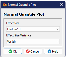
The vertical dotted line represents a quantile of zero; the horizontal dotted line represents the mean standardized effect size. The dashed lines represent the prediction confidence interval of the regression line. The width of the prediction envelope can be modified by choosing a different significance level from the output options.
Output Example
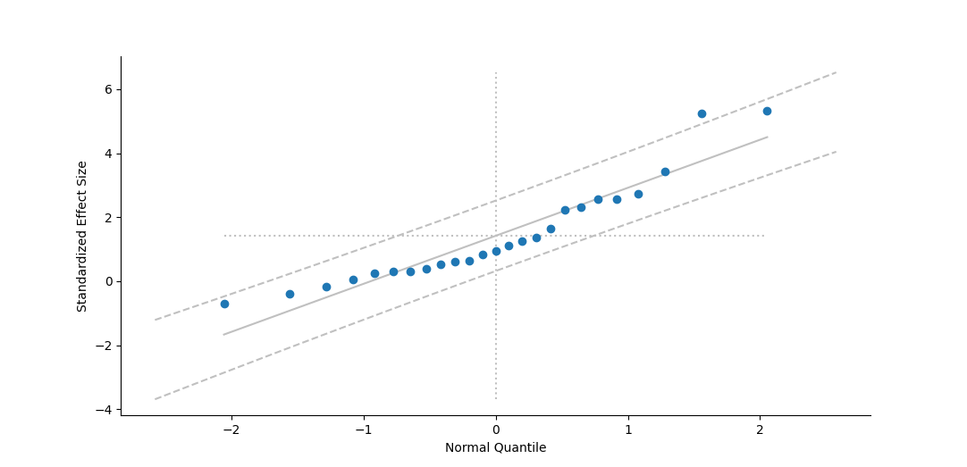
Normal Quantile plot following Wang and Bushman (1998). The standardized effect size is the effect size divided by the square-root of its variance. The solid line represents the regression and the dashed lines the 95% prediction envelope.
References
Wang, M.C., and B.J. Bushman (1998) Using the normal quantile plot to explore meta-analytic data sets. Psychological Methods 3:46–54.
Galbraith (Radial) Plot
A Galbraith Plot (also known as a Radial Plot) is a special type of scatter plot where a measure of precision (the square-root of the variance) is plotted on the x-axis and a standardized effect size (the effect size × precision) is plotted on the y-axis. A straight line drawn from the origin through any point, intersects a curve on the right side of the plot with the magnitude of the effect size, and the regression of the points through the origin intersects the curve at the mean effect size. See Galbraith (1988, 1994) for more details.
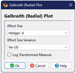
To draw a Galbraith plot, choose from the menu. From here you can specify the Effect Size and Variance. Optionally you can also specify whether the Effect Size is a log-transformed measure; if you do so the values indicated on the resulting radial arc will be displayed using "unlogged" ratios.
Output Example
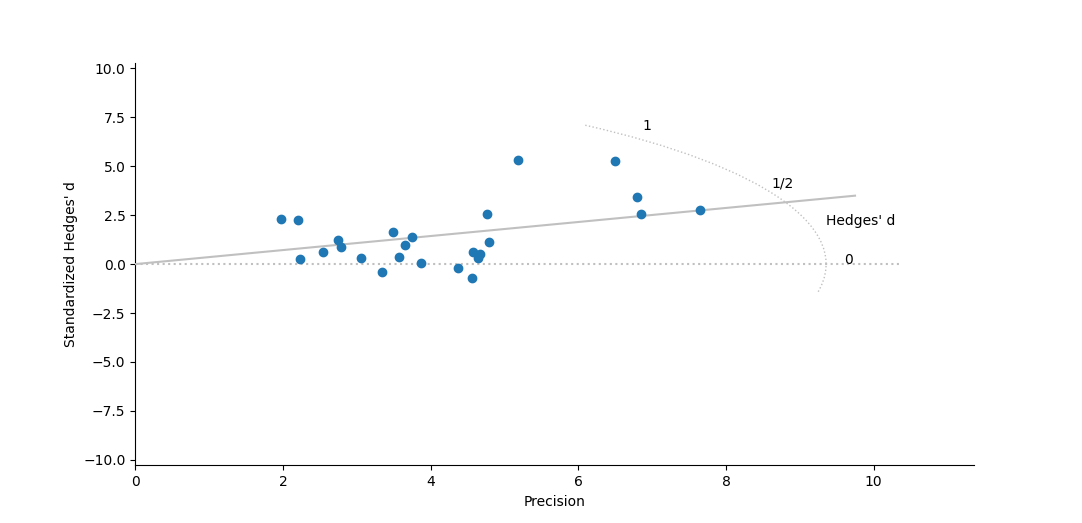
Radial chart (Galbraith 1988, 1994) of standardized Hedges' d vs. precision. A line from the origin through any point intersects the curve at the effect size for that point. The regression line intersects the curve at the mean effect size.
References
Galbraith, R.F. (1988) A note on graphical presentation of estimated odds ratios from several clinical trials. Statistics in Medicine 7:889–894.
Galbraith, R.F. (1994) Some applications of radial plots. Journal of the American Statistical Association 89:1232–1242.
References
- Adams, D.C., J. Gurevitch, and M.S. Rosenberg (1997) Resampling tests for meta-analysis of ecological data. Ecology 78(4):1277–1283. DOI: 10.1890/0012-9658(1997)078[1277:RTFMAO]2.0.CO;2
- Begg, C.B. (1994) Publication bias. Pp. 399-409 in The Handbook of Research Synthesis, H. Cooper and L.V. Hedges, eds. Sage, New York.
- Begg, C.B., and M. Mazumdar (1994) Operating characteristics of a rank correlation test for publication bias. Biometrics 50:1088–1101. DOI: 10.2307/2533446
- Berlin, J.A., N.M. Laird, H.S. Sacks, and T.C. Chalmers (1989) A comparison of statistical methods for combining event rates from clinical trials. Statistics in Medicine 8:141–151. DOI: 10.1002/sim.4780080202
- Chalmers, T.C. (1991) Problems induced by meta-analyses. Statistics in Medicine 10:971–980. DOI: 10.1002/sim.4780100618
- DerSimonian, R., and N. Laird (1986) Meta-analysis in clinical trials. Controlled Clinical Trials 7:177–188. DOI: 10.1016/0197-2456(86)90046-2
- Duval, S. and R. Tweedie (2000a) A nonparametric "trim and fill" method of accounting for publication bias in meta-analysis. Journal of the American Statistical Association 95(449):89–98. DOI: 10.1080/01621459.2000.10473905
- Duval, S. and R. Tweedie (2000b) Trim and fill: A simple funnel-plot-based method of testing and adjusting for publication bias in meta-analysis. Biometrics 56:455–463. DOI: 10.1111/j.0006-341X.2000.00455.x
- Egger, M., G.D. Smith, M. Schneider, and C. Minder (1997) Bias in meta-analysis detected by a simple, graphical test. BMJ 315:629–634. DOI: 10.1136/bmj.315.7109.629
- Fisher, R.A. (1928) Statistical methods for research workers (2nd edition). Oliver and Boyd, London.
- Galbraith, R.F. (1988) A note on graphical presentation of estimated odds ratios from several clinical trials. Statistics in Medicine 7:889–894. DOI: 10.1002/sim.4780070807
- Galbraith, R.F. (1994) Some applications of radial plots. Journal of the American Statistical Association 89:1232–1242. DOI: 10.1080/01621459.1994.10476864
- Greenland, S. (1987) Quantitative methods in the review of epidemiologic literature. Epidemiologic Review 9:1–30. DOI: 10.1093/oxfordjournals.epirev.a036298
- Hedges, L.V. and I. Olkin (1985) Statistical Methods for Meta-analysis. Academic Press, Orlando, FL.
- Hedges, L.V., J. Gurevitch, and P.S. Curtis (1999) The meta-analysis of response ratios in experimental ecology. Ecology 80(4):1150–1156. DOI: 10.1890/0012-9658(1999)080[1150:TMAORR]2.0.CO;2
- Higgins, J.P.T. and S.G. Thompson (2002) Quantifying heterogeneity in a meta-analysis. Statistics in Medicine 21:1539–1558. DOI: 10.1002/sim.1186
- Huedo-Medina, T.B., J. Sánchez-Meca, F. Marín-Martínez, and J. Botella (2006) Assessing heterogeneity in meta-analysis: Q statistic or I2 index? Psychological Methods 11:193–206. DOI: 10.1037/1082-989X.11.2.193
- Kendall, M. (1938) A new measure of rank correlation. Biometrika. 30(1–2):81–89. DOI: 10.1093/biomet/30.1-2.81
- Kossmeier, M., U.S. Tran, and M. Voracek (2020) Power-enhanced funnel plots for meta-analysis: The sunset funnel plot. Zeitschrift für Psychologie 228(1):43–49. DOI: 10.1027/2151-2604/a000392
- L’Abbé, K.A., A.S. Detsky, and K. O’Rourke (1987) Meta-analysis in clinical research. Annals of Internal Medicine 107:224–233. DOI: 10.7326/0003-4819-107-2-224
- Lajeunesse, M.J. (2009) Meta-analysis and the comparative phylogenetic method. American Naturalist 174:369–381. DOI: 10.1086/603628
- Lajeunesse, M.J., M.S. Rosenberg, and M.D. Jennions (2013) Phylogenetically independent meta-analysis. Pp. 284–299 in Handbook of Meta-analysis in Ecology and Evolution, J. Koricheva, J. Gurevitch and K.L. Mengersen, eds. Princeton University Press: Princeton, NJ. DOI: 10.23943/princeton/9780691137285.003.0017
- Light, R.J., and D.B. Pillemer (1984) Summing Up: The Science of Reviewing Research. Harvard University Press: Cambridge.
- Mantel, N., and W. Haenszel (1959) Statistical aspects of the analysis of data from retrospective studies of disease. Journal of the National Cancer Institute 22:719–748. DOI: 10.1093/jnci/22.4.719
- Mengersen, K., and J. Gurevitch (2013) Using other metrics of effect size in meta-analysis. Pp. 72–85 in Handbook of Meta-analysis in Ecology and Evolution, J. Koricheva, J. Gurevitch and K.L. Mengersen, eds. Princeton University Press: Princeton, NJ. DOI: 10.23943/princeton/9780691137285.003.0007
- Nakagawa, S., M. Lagisz, M.D. Jennions, J. Koricheva, D.W.A. Noble, T.H. Parker, A. Sánchez-Tójar, Y. Yang, and R.E. O'Dea (2022) Methods for testing publication bias in ecological and evolutionary meta-analyses. Methods in Ecology and Evolution 13(1):4–21. DOI: 10.1111/2041-210X.13724
- Normand, S.-L.T. (1999) Meta-analysis: Formulating, evaluating, combining, and reporting. Statistics in Medicine 18:321—359. DOI: 10.1002/(sici)1097-0258(19990215)18:3<321::aid-sim28>3.0.co;2-p
- Orwin, R.G. (1983) A fail-safe N for effect size in meta-analysis. Journal of Educational Statistics 8(2):157–159. DOI: 10.2307/1164923
- Peters, J.L., A.J. Sutton, D.R. Jones, K.R. Abrams, and L. Rushton (2008) Contour-enhanced meta-analysis funnel plots help distinguish publication bias from other causes of asymmetry. Journal of Clinical Epidemiology 61(10):991–996. 10.1016/j.jclinepi.2007.11.010
- Rosenberg, M.S. (2005) The file-drawer problem revisited: A general weighted method for calculating fail-safe numbers in meta-analysis. Evolution 59(2):464–468. DOI: 10.1554/04-602
- Rosenberg, M.S. (2024) MetaWin 3: Open-source software for meta-analysis. Frontiers in Bioinformatics 4:1305969. DOI: 10.3389/fbinf.2024.1305969
- Rosenberg, M.S. (2013) Moment and least-squares based approaches to meta-analytic inference. Pp. 108–124 in Handbook of Meta-analysis in Ecology and Evolution, J. Koricheva, J. Gurevitch and K.L. Mengersen, eds. Princeton University Press: Princeton, NJ. DOI: 10.23943/princeton/9780691137285.003.0009
- Rosenberg, M.S., D.C. Adams, and J. Gurevitch (1997) MetaWin: Statistical Software for Meta-Analysis with Resampling Tests. Version 1. Sinauer Associates: Sunderland, MA.
- Rosenberg, M.S., D.C. Adams, and J. Gurevitch (2000) MetaWin: Statistical Software for Meta-Analysis. Version 2. Sinauer Associates: Sunderland, MA.
- Rosenthal, R. (1979) The “file drawer problem” and tolerance for null results. Psychological Bulletin 86(3):638–641. DOI: 10.1037/0033-2909.86.3.638
- Sokal, R.R., and F.J. Rohlf (1995) Biometry: The Principles and Practice of Statistics in Biological Research. 3rd edition. W.H. Freeman, New York.
- Spearman C. (1904) The proof and measurement of association between two things. American Journal of Psychology. 15(1):72–101. DOI: 10.2307/1412159
- Sterne, J.A.C., and M. Egger (2001) Funnel plots for detecting bias in meta-analysis: Guidelines on choice of axis. Journal of Clinical Epidemiology 54(10):1045–1055. DOI: 10.1016/S0895-4356(01)00377-8
- Wang, M.C., and B.J. Bushman (1998) Using the normal quantile plot to explore meta-analytic data sets. Psychological Methods 3:46–54. DOI: 10.1037/1082-989X.3.1.46